rcs generates bad prediction in lm() models

Question

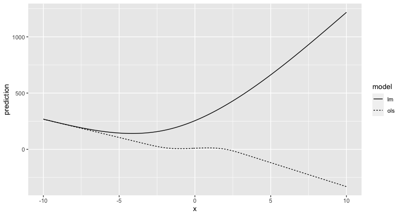
I'm trying to reproduce this blog post on overfitting. I want to explore how a spline compares to the tested polynomials.

My problem: Using the rcs() - restricted cubic splines - from the rms package I get very strange predictions when applying in regular lm(). The ols() works fine but I'm a little surprised by this strange behavior. Can someone explain to me what's happening?

library(rms)
p4 <- poly(1:100, degree=4)
true4 <- p4 %*% c(1,2,-6,9)
days <- 1:70

noise4 <- true4 + rnorm(100, sd=.5)
reg.n4.4 <- lm(noise4[1:70] ~ poly(days, 4))
reg.n4.4ns <- lm(noise4[1:70] ~ ns(days,5))
reg.n4.4rcs <- lm(noise4[1:70] ~ rcs(days,5))
dd <- datadist(noise4[1:70], days)
options("datadist" = "dd")
reg.n4.4rcs_ols <- ols(noise4[1:70] ~ rcs(days,5))

plot(1:100, noise4)
nd <- data.frame(days=1:100)
lines(1:100, predict(reg.n4.4, newdata=nd), col="orange", lwd=3)
lines(1:100, predict(reg.n4.4ns, newdata=nd), col="red", lwd=3)
lines(1:100, predict(reg.n4.4rcs, newdata=nd), col="darkblue", lwd=3)
lines(1:100, predict(reg.n4.4rcs_ols, newdata=nd), col="grey", lwd=3)

legend("top", fill=c("orange", "red", "darkblue", "grey"), 
       legend=c("Poly", "Natural splines", "RCS - lm", "RCS - ols"))

As you can see the darkblue is allover the place...

Buttery

rcs is not designed to work with lm - why do you expect it to? – Otherworld

@hadley: I'm aware that it is not designed for lm. I just thought that all the splines, polynomials etc were just transforming a vector into a matrix and that it isn't that package specific. – Buttery

Answer 1

You can use rcs() with non-rms fitters as long as you specify the knots. predict defaults to predict.ols for an ols object, which is nice because it "remembers" where it put the knots when it fit the model. predict.lm does not have that functionality, so it uses the distribution of the new data set to determine the placement of the knots, rather than the distribution of the training data.

Bean

Answer 2

Using lm with rcs is a bad idea, even if you specify the knots in rcs. Here's an example:

Fake data.

library(tidyverse)
library(rms)

set.seed(100)

xx <- rnorm(1000)
yy <- 10 + 5*xx - 0.5*xx^2 - 2*xx^3 + rnorm(1000, 0, 4)
df <- data.frame(x=xx, y=yy)

Setup your environment to use ols.

ddist <- datadist(df)
options("datadist" = "ddist")

Fit lm model and ols model.

mod_ols <- ols(y ~ rcs(x, parms=c(min(x), -2, 0, 2, max(x))), data=df)

mod_lm <- lm(y ~ rcs(x, parms=c(min(x),-2, 0, 2, max(x))), data=df)

Create a test data set.

newdf <- data.frame(x=seq(-10, 10, 0.1))

Compare the model predictions after scoring newdf.

preds_ols <- predict(mod_ols, newdata=newdf)
preds_lm <- predict(mod_lm, newdata=newdf)

mean((preds_ols - preds_lm)^2)

as.numeric(coef(mod_ols))
as.numeric(coef(mod_lm))

compare_df <- newdf
compare_df$ols <- preds_ols
compare_df$lm <- preds_lm

compare_df <- compare_df %>% 
  gather(key="model", value="prediction", -x)

ggplot(compare_df, aes(x=x, y=prediction, group=model, linetype=model)) +
  geom_line()

The model predictions can be different on new data, even though the coefficients are identical between the two models.

Edit:

Removing the function calls to max() and min(), in the parms argument, solves the issue.

kKnots <- with(df, c(min(x), -2, 0, 2, max(x))) ## hard-code

mod_ols <- ols(y ~ rcs(x, parms=kKnots), data=df)

mod_lm <- lm(y ~ rcs(x, parms=kKnots), data=df)

Youngstown