Map of bivariate spatial correlation in R (bivariate LISA)

Question

I would like to create a map showing the bi-variate spatial correlation between two variables. This could be done either by doing a LISA map of bivariate Moran's I spatial correlation or using the L index proposed by Lee (2001).

The bi-variate Moran's I is not implemented in the spdep library, but the L index is, so here is what I've tried without success using the L index. A answer showing a solution based on Moran's I would also be very welcomed !

As you can see from the reproducible example below, I've manged so far to calculate the local L indexes. What I would like to do is to estimate the pseudo p-values and create a map of the results like those maps we use in LISA spatial clusters with high-high, high-low, ..., low-low.

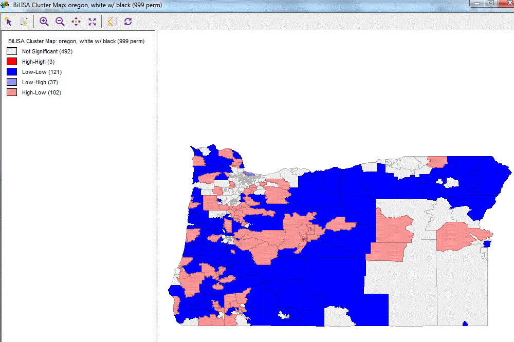
In this example, the goal is to create a map with bi-variate Lisa association between black and white population. The map should be created in ggplot2 , showing the clusters:

• High-presence of black and High-presence of white people
• High-presence of black and Low-presence of white people
• Low-presence of black and High-presence of white people
• Low-presence of black and Low-presence oh white people

Reproducible example

library(UScensus2000tract)
library(ggplot2)
library(spdep)
library(sf)

# load data
  data("oregon.tract")

# plot Census Tract map
  plot(oregon.tract)


# Variables to use in the correlation: white and black population in each census track
  x <- scale(oregon.tract$white)
  y <- scale(oregon.tract$black)


# create  Queen contiguity matrix and Spatial weights matrix
  nb <- poly2nb(oregon.tract)
  lw <- nb2listw(nb)


# Lee index
  Lxy <-lee(x, y, lw, length(x), zero.policy=TRUE)

  # Lee’s L statistic (Global)
    Lxy[1]
    #> -0.1865688811


# 10k permutations to estimate pseudo p-values
  LMCxy <- lee.mc(x, y, nsim=10000, lw, zero.policy=TRUE, alternative="less")

# quik plot of local L
  Lxy[[2]] %>% density() %>% plot() # Lee’s local L statistic  (Local)
  LMCxy[[7]] %>% density() %>% lines(col="red") # plot values simulated 10k times 


# get confidence interval of 95% ( mean +- 2 standard deviations)
  two_sd_above <- mean(LMCxy[[7]]) + 2 * sd(LMCxy[[7]])
  two_sd_below <- mean(LMCxy[[7]]) - 2 * sd(LMCxy[[7]])


# convert spatial object to sf class for easier/faster use
  oregon_sf <- st_as_sf(oregon.tract)


# add L index values to map object
  oregon_sf$Lindex <- Lxy[[2]]

# identify significant local results  
  oregon_sf$sig <- if_else( oregon_sf$Lindex < 2*two_sd_below, 1, if_else( oregon_sf$Lindex > 2*two_sd_above, 1, 0))


# Map of Local L index but only the significant results
  ggplot() + geom_sf(data=oregon_sf, aes(fill=ifelse( sig==T, Lindex, NA)), color=NA)

Autarch

Answer 1

What about this?

I'm using the regular Moran's I instead of that Lee Index you suggest. But I think the underlying reasoning is pretty much the same.

As you may see bellow -- the results produced this way look very much alike those comming from GeoDA

library(dplyr)
library(ggplot2)
library(sf)
library(spdep)
library(rgdal)
library(stringr)
library(UScensus2000tract)

#======================================================
# load data
data("oregon.tract")

# Variables to use in the correlation: white and black population in each census track
x <- oregon.tract$white
y <- oregon.tract$black

#======================================================
# Programming some functions

# Bivariate Moran's I
moran_I <- function(x, y = NULL, W){
        if(is.null(y)) y = x

        xp <- (x - mean(x, na.rm=T))/sd(x, na.rm=T)
        yp <- (y - mean(y, na.rm=T))/sd(y, na.rm=T)
        W[which(is.na(W))] <- 0
        n <- nrow(W)

        global <- (xp%*%W%*%yp)/(n - 1)
        local  <- (xp*W%*%yp)

        list(global = global, local  = as.numeric(local))
}


# Permutations for the Bivariate Moran's I
simula_moran <- function(x, y = NULL, W, nsims = 1000){

        if(is.null(y)) y = x

        n   = nrow(W)
        IDs = 1:n

        xp <- (x - mean(x, na.rm=T))/sd(x, na.rm=T)
        W[which(is.na(W))] <- 0

        global_sims = NULL
        local_sims  = matrix(NA, nrow = n, ncol=nsims)

        ID_sample = sample(IDs, size = n*nsims, replace = T)

        y_s = y[ID_sample]
        y_s = matrix(y_s, nrow = n, ncol = nsims)
        y_s <- (y_s - apply(y_s, 1, mean))/apply(y_s, 1, sd)

        global_sims  <- as.numeric( (xp%*%W%*%y_s)/(n - 1) )
        local_sims  <- (xp*W%*%y_s)

        list(global_sims = global_sims,
             local_sims  = local_sims)
}


#======================================================
# Adjacency Matrix (Queen)

nb <- poly2nb(oregon.tract)
lw <- nb2listw(nb, style = "B", zero.policy = T)
W  <- as(lw, "symmetricMatrix")
W  <- as.matrix(W/rowSums(W))
W[which(is.na(W))] <- 0

#======================================================
# Calculating the index and its simulated distribution
# for global and local values

m   <- moran_I(x, y, W)
m[[1]] # global value

m_i <- m[[2]]  # local values

local_sims <- simula_moran(x, y, W)$local_sims

# Identifying the significant values 
alpha <- .05  # for a 95% confidence interval
probs <- c(alpha/2, 1-alpha/2)
intervals <- t( apply(local_sims, 1, function(x) quantile(x, probs=probs)))
sig        <- ( m_i < intervals[,1] )  | ( m_i > intervals[,2] )

#======================================================
# Preparing for plotting

oregon.tract     <- st_as_sf(oregon.tract)
oregon.tract$sig <- sig


# Identifying the LISA patterns
xp <- (x-mean(x))/sd(x)
yp <- (y-mean(y))/sd(y)

patterns <- as.character( interaction(xp > 0, W%*%yp > 0) ) 
patterns <- patterns %>% 
        str_replace_all("TRUE","High") %>% 
        str_replace_all("FALSE","Low")
patterns[oregon.tract$sig==0] <- "Not significant"
oregon.tract$patterns <- patterns


# Plotting
ggplot() + geom_sf(data=oregon.tract, aes(fill=patterns), color="NA") +
        scale_fill_manual(values = c("red", "pink", "light blue", "dark blue", "grey95")) + 
        theme_minimal()

You can get results closer (but not identical) to that of GeoDa by making changes in the confidence interval (e.g. using 90% instead of 95%).

I suppose the remaining discrepancies come from a slightly different method of calculating the Moran's I. My version gives the same values of that function moran available in the package spdep. But GeoDa probably uses another approach.

Valora

Thanks so much Rogerio, this looks promising. Is y_s the spatially lagged y ? – Autarch

@rafa.pereira, y_s stands for "y simulated". The lagged y is obtained after multiplying it by the adjacency matrix: W%*%y_s – Valora

Hi @RogerioJB, do you how to get the global p-value of Moran's I in your function ? – Autarch

The function also gives sim values for the global index: simula_moran(x, y, W)$global_sims. You can obtain the p-value by calculating the proportion of sims which the absolute value is higher than the abs value of the actual index. But probably this proportion will be zero or very close to zero, once a correlation index reaches significance very fast as the number of observations grows. You can get more precise results by increasing the number of simulations - but it may cause a R breakdown due to lack of RAM memory (if you do more than a million it will probably happen) – Valora

There is another method. Visually, the distribution of the simulated values seems to be symmetrical and centered around zero. If it is Normal and if increasing the number of sims makes this resemblance even better (you will have to test for it), then you can use the usual procedure of dividing the observed statistics by its standard deviation (and play a pseudo-asymptotical game) – Valora

Ok, so I did what you said. Get all simulated global Moran: global_sims <- simula_moran(x, y, W)$global_sims and then estimated the proportion of simulated global values that are higher (in absolute value) than the actual index: sum(abs(global_sims) > abs( m[[1]][1] )) / length(global_sims) – Autarch

I've also increased the number of simulations from 1K to 10K. – Autarch

Im very intruiged by this. Thanks for the contribution. Do u have a clue on how to actually derive p-values from the CI for the local values? l tried to work my way back but for my testing, apparently with your functions the local I values and the significance levels are correct, but the p-values I try to generate do not match up even remotely. – Congeneric

Answer 2

I suppose this is quite late to add to the thread, however Lee's L is quite different to what you have done here, which is Wartenberg's (1985) innovation. This has some potential drawbacks. Mainly, that it tests the relationship between x and the lag of y as @RogerioJB clarified by explaining that the spatially lagged y is calculated by multiplying the simulated y by the adjacency matrix. Lee's (2001) innovation is quite different and involves the integration of Pearson's r and a Spatial Smoothing Scalar (SSS) and instead compares the process between x and y as opposed to the lag of y. The approach @RogerioJB adopted can be replicated by generating the distribution of possible local l's from the lee.mc function. In turn the results can be plotted in a style that is similar to the GeoDa-like high-high ... low-low significance cluster map.

Easily

Answer 3

Building upon the suggestion by @justin-k, I modified the bivariate LISA code by @rogeriojb to calculate Lee's L statistic. This approach creates a modified lee.mc() function from the spdep package to simulate the local L values. I provide another example in a GitHub gist with point-level data.

library(boot)
library(dplyr)
library(ggplot2)
library(sf)
library(spdep)
library(rgdal)
library(stringr)
library(UScensus2000tract)

#======================================================
# load data
data("oregon.tract")

# Variables to use in the correlation: white and black population in each census track
x <- oregon.tract$white
y <- oregon.tract$black

# ----------------------------------------------------- #
# Program a function
## Permutations for Lee's L statistic
## Modification of the lee.mc() function within the {spdep} package
## Saves 'localL' output instead of 'L' output
simula_lee <- function(x, y, listw, nsim = nsim, zero.policy = NULL, na.action = na.fail) {
  
  if (deparse(substitute(na.action)) == "na.pass") 
    stop ("na.pass not permitted")
  na.act <- attr(na.action(cbind(x, y)), "na.action")
  x[na.act] <- NA
  y[na.act] <- NA
  x <- na.action(x)
  y <- na.action(y)
  if (!is.null(na.act)) {
    subset <- !(1:length(listw$neighbours) %in% na.act)
    listw <- subset(listw, subset, zero.policy = zero.policy)
  }
  n <- length(listw$neighbours)
  if ((n != length(x)) | (n != length(y))) 
    stop ("objects of different length")
  gamres <- suppressWarnings(nsim > gamma(n + 1))
  if (gamres) 
    stop ("nsim too large for this number of observations")
  if (nsim < 1) 
    stop ("nsim too small")
  xy <- data.frame(x, y)
  S2 <- sum((unlist(lapply(listw$weights, sum)))^2)
  
  lee_boot <- function(var, i, ...) {
    return(lee(x = var[i, 1], y = var[i, 2], ...)$localL)
  }
  
  res <- boot(xy, statistic = lee_boot, R = nsim, sim = "permutation", 
              listw = listw, n = n, S2 = S2, zero.policy = zero.policy)
}

# ----------------------------------------------------- #
# Adjacency Matrix
nb <- poly2nb(oregon.tract)
lw <- nb2listw(nb, style = "B", zero.policy = T)
W  <- as(lw, "symmetricMatrix")
W  <- as.matrix(W / rowSums(W))
W[which(is.na(W))] <- 0

# ----------------------------------------------------- #
# Calculate the index and its simulated distribution
# for global and local values

# Global Lee's L
lee.test(x = x, y = y, listw = lw, zero.policy = TRUE,
         alternative = "two.sided", na.action = na.omit)

# Local Lee's L values
m <- lee(x = x, y = y, listw = lw, n = length(x), 
         zero.policy = TRUE, NAOK = TRUE)

# Local Lee's L simulations
local_sims <- simula_lee(x = x, y = y, listw = lw, nsim = 10000,
                         zero.policy = TRUE, na.action = na.omit)

m_i <- m[[2]]  # local values

# Identify the significant values 
alpha <- 0.05  # for a 95% confidence interval
probs <- c(alpha/2, 1-alpha/2)
intervals <- t(apply(t(local_sims[[2]]), 1, function(x) quantile(x, probs = probs)))
sig <- (m_i < intervals[ , 1] ) | ( m_i > intervals[ , 2])

#======================================================
# Preparing for plotting
oregon.tract <- st_as_sf(oregon.tract)
oregon.tract$sig <- sig

# Identifying the Lee's L patterns
xp <- scale(x)
yp <- scale(y)

patterns <- as.character(interaction(xp > 0, W%*%yp > 0)) 
patterns <- patterns %>% 
  str_replace_all("TRUE","High") %>% 
  str_replace_all("FALSE","Low")
patterns[oregon.tract$sig == 0] <- "Not significant"
oregon.tract$patterns <- patterns

# Plotting
ggplot() +
  geom_sf(data = oregon.tract, aes(fill = patterns), color = "NA") +
  scale_fill_manual(values = c("red", "pink", "light blue", "dark blue", "grey95")) + 
  guides(fill = guide_legend(title = "Lee's L clusters")) +
  theme_minimal()

Lee's L clusters for oregon.tract data

Sturges