Multiple, dependent-level sunburst/doughnut chart using ggplot2

Question

I'm trying to create a two-level sunburst/doughnut diagram (for print) where the second level is a detailed view of the first. I've read and understood this tutorial, but I'm an R and ggplot2 newbie and am having trouble producing the second level. In the aforementioned article, the root level only has one element (which is a bit redundant), whereas my root has many elements; of which, the secondary level has at least 1 and up to 10 elements.

Let's say my data has three columns: name, type and value; where name and type define the root and second level elements, respectively. Each name has exactly one type of all, which is the summation of the values across over types (of which, there's at least one and, across names the sets of type may intersect or be mutually exclusive). For example:

name  type    value
----- ------- ------
foo   all     444
foo   type1   123
foo   type2   321
bar   all     111
bar   type3   111
baz   all     999
baz   type1   456
baz   type3   543

I can create the root level stack (before being converted to polar coordinates) using:

data.all <- data[data$type == "all",]
ggplot(data.all, aes(x=1, y=data.all$value, fill=data.all$name)) + geom_bar(stat="identity")

What I need for the second level stack is for the type values to align within the name values, proportional to their value:

 +-----+  +-------+
 |     |  | type3 |
 | baz |  +-------+
 |     |  | type1 |
 +-----+  +-------+
 |     |  |       |
 | bar |  | type3 |
 |     |  |       |
 +-----+  +-------+
 |     |  | type2 |
 | foo |  +-------+
 |     |  | type1 |
-+-----+--+-------+-

(n.b., this is obviously not to scale!)

I also need the type values to be coloured consistently (e.g., the colour of the type1 block should be the same for both foo and baz, etc.)

I thought I could do this by combining the name and type columns into a new column and then colouring by this:

data.other <- data[data$type != "other",]
data.other$comb <- paste(data.other$name, data.other$type, sep=":")
ggplot(data.other, aes(x=2, y=data.other$value, fill=data.other$comb)) + geom_bar(stat="identity")

However, this breaks the colouring consistency -- obviously, in hindsight -- and, anecdotally, I have absolutely no faith that the alignment will be correct.

My R/ggplot2 nativity is probably pretty apparent (sorry!); how can I achieve what I'm looking for?

---

EDIT I also came across this question and answer, however my data looks different to theirs. If my data can be munged into the same shape -- which I don't know how to do -- then my question becomes a special case of theirs.

Callboy

Possible duplicate of How to make a sunburst plot in R or Python? – Messidor

There's a package ggsunburst if you want to avoid doing it from scratch – Messidor

@Messidor Just having a play with ggsunburst and it appears to only support tree structures with non-weighted nodes. sunburstR looks like it produces interactive, web-based output, rather than something static for print (e.g., a PDF) – Callboy

Okay. I suppose you don't want to change your data into a tree? (It's cool if you don't.) Is the data sample you posted above everything you're working with? If not, could you dput your data? – Messidor

The data in my question is an illustrative example to show the structure; my real data is far more complicated and much, much bigger (and generated from an external source), such that it wouldn't be appropriate to spew out into SO. The salient parts are isomorphic to my example: name and type denote the levels (with a special type of all, for convenience) and value weights the nodes (where the value of the all type is the sum of the other types for each name). – Callboy

Answer 1

This might only be partway there, and it might not scale well to a much more complex dataset. I got intensely curious about how to do this, and had a similar larger dataset I'm trying to visualize for work, so this is actually helping my out with my job too :)

Basically what I did is split the dataset into dataframes for three levels: a parent level that's basically dummy data, a level 1 df with sums of all the types under each name (I suppose I could have just filtered your data for type == "all"--I didn't have a similar column for my work data), and a level 2 that's all the outer nodes. Bind them all together, make a stacked bar chart, give it polar coordinates.

The one I did for work had a lot more labels, and they were pretty long, so I used ggrepel::geom_text_repel for the labels instead. They quickly became unwieldy and ugly.

Obviously the aesthetics here leave something to be desired, but I think it could be beautified to your liking.

library(tidyverse)

df <- "name  type    value
foo   all     444
foo   type1   123
foo   type2   321
bar   all     111
bar   type3   111
baz   all     999
baz   type1   456
baz   type3   543" %>% read_table2() %>%
    filter(type != "all") %>%
    mutate(name = as.factor(name) %>% fct_reorder(value, sum)) %>%
    arrange(name, value) %>%
    mutate(type = as.factor(type) %>% fct_reorder2(name, value))

lvl0 <- tibble(name = "Parent", value = 0, level = 0, fill = NA)

lvl1 <- df %>%
    group_by(name) %>%
    summarise(value = sum(value)) %>%
    ungroup() %>%
    mutate(level = 1) %>%
    mutate(fill = name)

lvl2 <- df %>%
    select(name = type, value, fill = name) %>%
    mutate(level = 2)


bind_rows(lvl0, lvl1, lvl2) %>%
    mutate(name = as.factor(name) %>% fct_reorder2(fill, value)) %>%
    arrange(fill, name) %>%
    mutate(level = as.factor(level)) %>%
    ggplot(aes(x = level, y = value, fill = fill, alpha = level)) +
        geom_col(width = 1, color = "gray90", size = 0.25, position = position_stack()) +
        geom_text(aes(label = name), size = 2.5, position = position_stack(vjust = 0.5)) +
        coord_polar(theta = "y") +
        scale_alpha_manual(values = c("0" = 0, "1" = 1, "2" = 0.7), guide = F) +
        scale_x_discrete(breaks = NULL) +
        scale_y_continuous(breaks = NULL) +
        scale_fill_brewer(palette = "Dark2", na.translate = F) +
        labs(x = NULL, y = NULL) +
        theme_minimal()

Created on 2018-04-24 by the reprex package (v0.2.0).

Messidor

This is really close to what I'm looking for and it works with my data; thanks for going to so much trouble :) Your technique seems to only work if the colours of the outer band match those of the inner band, however I can probably work around this – Callboy

Cool, I think you could adjust how the colors are set. I did it this way because I've usually seen sunbursts with the color based on a parent group, then either lighter or less opaque as you go out from the center, but no need to do it only that way. – Messidor

What I was looking for is to use a distinct palette for the inner and outer rings, respectively. I'm not sure how to do that, or even if it's possible. My outer ring sectors can be very small, so labels get messy. I've sort-of-not-really got a solution by using the alpha channel as the secondary palette; it's not quite distinctive enough, but good enough to give an impression. – Callboy

I think that's possible. You might just need to mess with a manual color palette. I'm having a hard time hacking together the factors in the right order so groups stay together, with changing the coloring though – Messidor

Likewise! It seems every time you try to use the secondary level as the fill factor, it reorders everything and doesn’t respect any subsequent arrange calls. – Callboy

Unlike other sunburst examples on the web, this actually works (in 2022). Thank you. – Cockspur

Answer 2

It can be done with ggsunburst (as camille suggested). ggsunburst reads both newick and csv (or any delimiter-separated) files. You will need to install the latest version 0.0.9 in order for this example to work

# first row with header is mandatory
# remove lines with type "all" from your data
# add colour as additional column
df <- read.table(header=T, text =
"parent node  size  colour
foo   type1   123 type1
foo   type2   321 type2
bar   type3   111 type3
baz   type1   456 type1
baz   type3   543 type3")

# write data.frame into csv file
write.table(df, file = 'df.csv', row.names = F, sep = ",")

# install ggsunburst 0.0.9
if (!require("ggplot2")) install.packages("ggplot2")
if (!require("rPython")) install.packages("rPython")
install.packages("http://genome.crg.es/~didac/ggsunburst/ggsunburst_0.0.9.tar.gz", repos=NULL, type="source")


library(ggsunburst)

sb <- sunburst_data('df.csv', type = "node_parent", sep = ',', node_attributes = 'colour')
sunburst(sb, rects.fill.aes = "colour", node_labels = T, node_labels.min = 25)

see your sunburst here

Durwin

Answer 3

I was looking for a way to do this type of plot using ggplot. @camille answer was really helpful! I ended up using this answer here too to create a slightly modified answer to this question.

It has been almost a year, but maybe someone else is still looking for this type of answer! Maybe the other packages mentioned in the other answers are more useful, but for those of us who want to stay within ggplot, hopefully this can help.

I think i could do what the OP was asking for (colouring the second level consistently) although I am not sure it is the optimal way to go.

Instead of using geom_col, I used geom_rect. This gives us more flexibility and also more control of where each rectangle is being drawn (stacked bars always have this issue of the order bars are stacked). Also, weirdly, in polar coord geom_col ends up drawing all the pies from 0 to x. So @camille had to play around with the transparencies of the fills in order to get the desired result. In geom_rect we can set xmin and xmax in order to get the exact shape we want.

But we need to do some data crunching to get the dataframes in shape.

Also, the plot I am trying to make has some of the second levels empty. So I changed the dataset a little to include one additional first level class without a second level class.

Here is my solution:

library(tidyverse)
library(ggplot2)
library(RColorBrewer)

df <- "name  type    value
foo   all     444
foo   type1   123
foo   type2   321
bar   all     111
bar   type3   111
baz   all     999
baz   type1   456
baz   type3   543
boz   -       222" %>% read_table2() %>% filter(type != 'all') %>% 
mutate(type=ifelse(type=='-', NA, type)) %>% arrange(name, value)

# here I create the columns xmin, xmax, ymin, ymax using cumsum function
# (be VERY careful with ordering of rows!)

# I also created a column 'colour' which I map to the asthetic 'colour' (colour of line of each rectangle)
# it is a boolean saying if a line should or should not be drawn.
# for empty second levels i want to draw an empty space (no fill and no line)

# define a padding space between the levels of the pie chart 
padding <- 0.05

# create df for level 0
lvl0 <- tibble(name = "Parent", value = 0, level = 0, fill = NA) %>%
  mutate(xmin=0, xmax=1, ymin=0, ymax=value) %>%
  mutate(x.avg=0, y.avg=0, colour=FALSE)

print(lvl0)

# create df for level 1
lvl1 <- df %>%
  group_by(name) %>%
  summarise(value = sum(value)) %>%
  ungroup() %>%
  mutate(level = 1) %>%
  mutate(fill = name) %>%
  mutate(xmin=1+padding, xmax=2, ymin=0, ymax=cumsum(value)) %>%
  mutate(ymin=lag(ymax, default=0),
         x.avg=(xmin+xmax)/2,
         y.avg=(ymin+ymax)/2,
         colour=TRUE)

print(lvl1)

# create df for level 2
lvl2 <- df %>%
  select(name = type, value, fill = name) %>%
  mutate(level = 2) %>%
  mutate(fill=paste0(fill, '_', name)) %>%
  mutate(xmin=2+padding, xmax=3, ymin=0, ymax=cumsum(value)) %>%
  mutate(ymin=lag(ymax, default=0),
         x.avg=(xmin+xmax)/2,
         y.avg=(ymin+ymax)/2,
         colour=ifelse(grepl('_NA', fill), FALSE, TRUE))

print(lvl2)

# this is my dirty workaround for defining the colours of levels 1 one 2 independently. Probably not the best way and 
# maybe it will not scale very well... But for this small data set it seemed to work...

# number of classes in each level (don't include NA)
n.classes.1 <- 4
n.classes.2 <- 3
n.classes.total <- n.classes.1 + n.classes.2

# get colour pallete for level 1
col.lvl1 <- brewer.pal(n.classes.total,"Dark2")[1:n.classes.1]
names(col.lvl1) <- as.character(unique(lvl1$name))

# get colour pallete for level 2 (don't include NA)
col.lvl2 <- brewer.pal(n.classes.total,"Dark2")[(n.classes.1+1):n.classes.total]
names(col.lvl2) <- as.character(unique(lvl2$name)[!is.na(unique(lvl2$name))])

# compile complete color pallete
fill.pallete <- c(col.lvl1)

for (l1 in as.character(unique(lvl1$name))) {
  for (l2 in as.character(unique(lvl2$name))) {
    if (!is.na(l2)) {
        name.type <- paste0(l1, '_', l2)
        aux <- col.lvl2[l2]
        names(aux) <- name.type
        fill.pallete <- c(fill.pallete, aux)        
    } else {
        # if level2 is NA, then assign transparent colour
        name.type <- paste0(l1, '_NA')
        aux <- NA
        names(aux) <- name.type
        fill.pallete <- c(fill.pallete, aux)        
    }
  }
}
print(fill.pallete)


# put all data frames together for ggplot

df.total <- bind_rows(lvl0, lvl1, lvl2) %>%
  mutate(name = as.factor(name) %>% fct_reorder2(fill, value)) %>%
  arrange(fill, name) %>%
  mutate(level = as.factor(level))

print(df.total)

# create plot (it helped me to look at the rectangular coordinates first before changing to polar!)

g <- ggplot(data=df.total, aes(fill = fill)) +
  geom_rect(aes(ymax=ymax, ymin=ymin, xmax=xmax, xmin=xmin, colour=colour), size = 0.1) +
  scale_fill_manual(values = fill.pallete, , guide = F, na.translate = FALSE) +
  scale_color_manual(values = c('TRUE'='gray20', 'FALSE'='#FFFFFF00'), 
                     guide = F, na.translate = FALSE) +
  geom_text(aes(x = x.avg, y = y.avg, label = name), size = rel(2.5)) +
  scale_x_discrete(breaks = NULL) +
  scale_y_continuous(breaks = NULL) +
  labs(x = NULL, y = NULL) +
  theme_minimal() +
  theme(panel.grid=element_blank()) + 
  coord_polar(theta = "y", start = 0, direction = -1)

print(g)

This is the resulting plot.

Ketubim

Answer 4

Based on your recommended web page, try the following:

library(ggplot2) 
library(dplyr) 
library(scales) 

toRead <- "name  type    value
foo   all     444
foo   type1   123
foo   type2   321
bar   all     111
bar   type3   111
baz   all     999
baz   type1   456
baz   type3   543"

data <- read.table(textConnection(toRead), header = TRUE)
closeAllConnections()



sum_total_value = sum(data$value)

firstLevel = data %>% summarize(total_value=sum(value))

sunburst_0 = ggplot(firstLevel) # Just a foundation
sunburst_1 = 
  sunburst_0 + 
  geom_bar(data=firstLevel, aes(x=1, y=total_value), fill='darkgrey', stat='identity') +
  geom_text(aes(x=1, y=sum_total_value/2, label=paste('Sum of all VALUE had', comma(total_value))), color='white')

sunburst_1
sunburst_1 + coord_polar('y')


sum_val = data %>% group_by(type) %>%
  summarize(total_value=sum(value)) %>%
  arrange(desc(total_value))


sunburst_2 <- sunburst_1 +
  geom_bar(data=sum_val,
           aes(x=2, y=total_value, fill=total_value),
           color='white', position='stack', stat='identity', size=0.6) + 
  geom_text(data=sum_val, aes(label=paste(type, total_value), x=2, y=total_value), position='stack')

sunburst_2

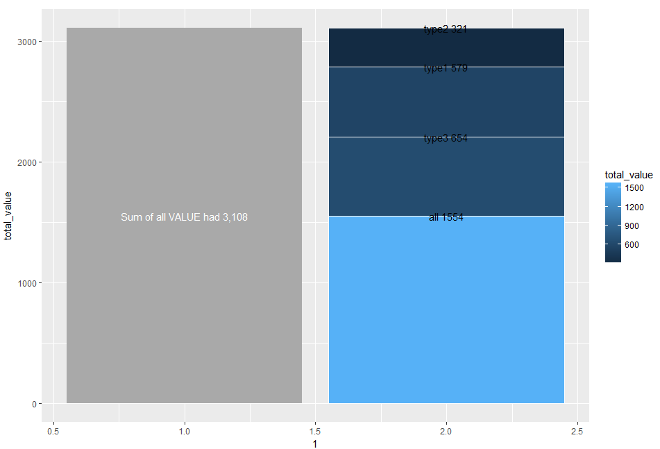
This gives the following plot:

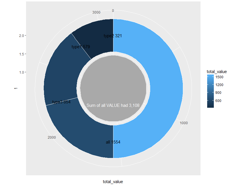
If you want this on polar coordinates, you can add the following:

sunburst_2 + coord_polar('y')

Which gives you:

Despotism

This sums all the values, across all names, as the root level (i.e., there's just one) and then the second level is split by type (including the special value of all, which by definition occupies exactly half the area). My question isn't about splitting the data by name or type exclusively, but by both simultaneously. The article has a single root level element, which is redundant in this kind of chart. A better example would be that in the question and answer mentioned in my edit, however their data is in a different form to mine. – Callboy

Absolutely. Glad to help. I am still not sure I understand what your desired output is. Is it: A.) just adding a second outer ring to the coordinate plot? or B.) creating a single level coordinate plot based on the combined values of the name and type values or C.) Something else... – Despotism

The point is that the outer ring is dependent upon the inner ring. As I say, if the inner ring only has one sector -- as in said article and your answer -- there is no point in doing this. In my example data, the inner ring would have three sectors and the outer ring would have 1 sector for bar and 2 sectors for foo and baz, all proportional to their values. – Callboy