I used your question to play a little with new libraries...
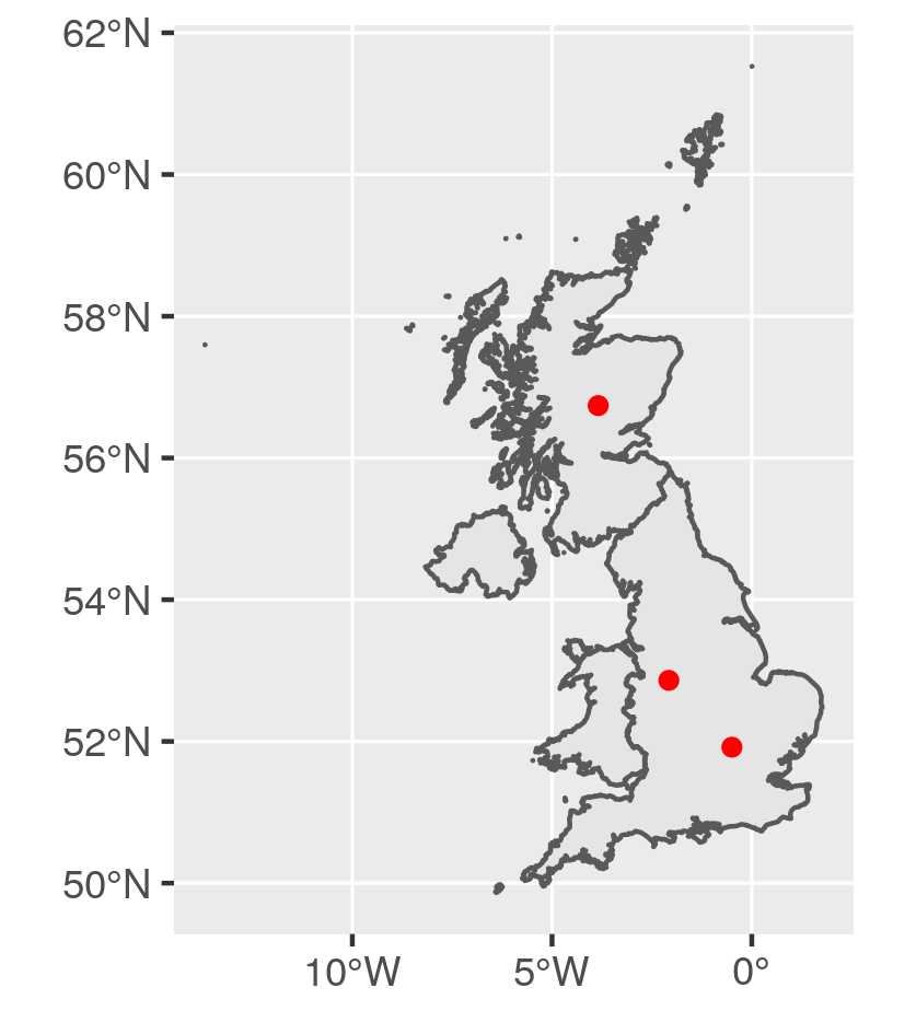
Get a UK map and define random points
library(raster)
library(sf)
library(ggplot2)
library(dplyr)
library(tidyr)
library(forcats)
library(purrr)

# Get UK map
GBR <- getData(name = "GADM", country = "GBR", level = 1)
GBR_sf <- st_as_sf(GBR)

# Define 3 points on the UK map
pts <- matrix(c(-0.4966766, -2.0772529, -3.8437793,
                51.91829, 52.86147, 56.73899), ncol = 2)
# Project in mercator to allow buffer with distances
pts_sf <- st_sfc(st_multipoint(pts), crs = 4326) %>%
  st_sf() %>%
  st_transform(27700)

ggplot() +
  geom_sf(data = GBR_sf) +
  geom_sf(data = pts_sf, colour = "red")
![Data Map]()
Calculate buffer areas
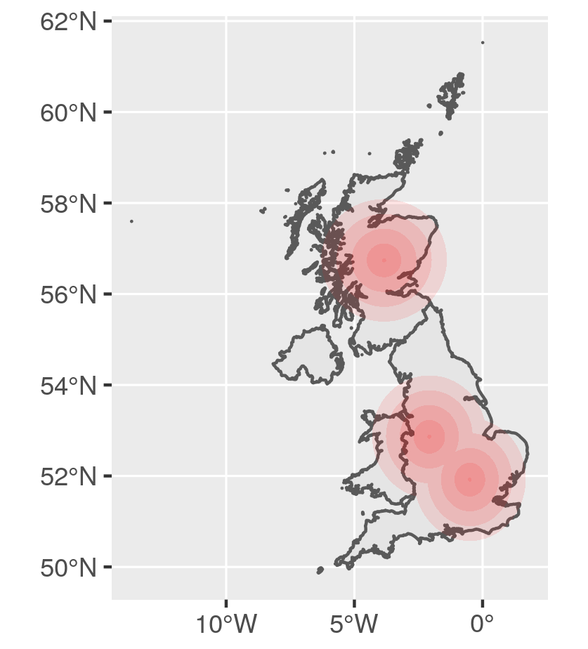
We create a list of multipolygons for each buffer distance. The point dataset must be in projected coordinates (here mercator) as buffer distance is in the scale of the coordinates system.
# Define distances to buffer
dists <- seq(5000, 150000, length.out = 5)
# Create buffer areas with each distances
pts_buf <- purrr::map(dists, ~st_buffer(pts_sf, .)) %>%
  do.call("rbind", .) %>%
  st_cast() %>%
  mutate(
    distmax = dists,
    dist = glue::glue("<{dists/1000} km"))
# Plot: alpha allows to see overlapping polygons
ggplot() +
  geom_sf(data = GBR_sf) +
  geom_sf(data = pts_buf, fill = "red",
          colour = NA, alpha = 0.1)
![Buffer overlap]()
Remove overlapping
Buffer areas are overlapping. On the figure above, the more intense red color is due to multiple overlapping layers of transparent red. Let's remove the overlapping. We need to remove from larger areas, the buffer with the lower size. I then need to add again the smallest area to the list.
# Remove part of polygons overlapping smaller buffer
pts_holes <- purrr::map2(tail(1:nrow(pts_buf),-1),
            head(1:nrow(pts_buf),-1),
            ~st_difference(pts_buf[.x,], pts_buf[.y,])) %>%
  do.call("rbind", .) %>%
  st_cast() %>%
  select(-distmax.1, -dist.1)
# Add smallest polygon
pts_holes_tot <- pts_holes %>%
  rbind(filter(pts_buf, distmax == min(dists))) %>%
  arrange(distmax) %>%
  mutate(dist = forcats::fct_reorder(dist, distmax))
# Plot and define color according to dist
ggplot() +
  geom_sf(data = GBR_sf) +
  geom_sf(data = pts_holes_tot,
          aes(fill = dist),
          colour = NA) +
  scale_fill_brewer(direction = 2)
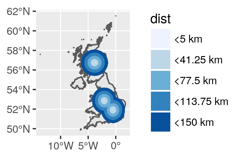
![Buffer with holes - donut polygons]()
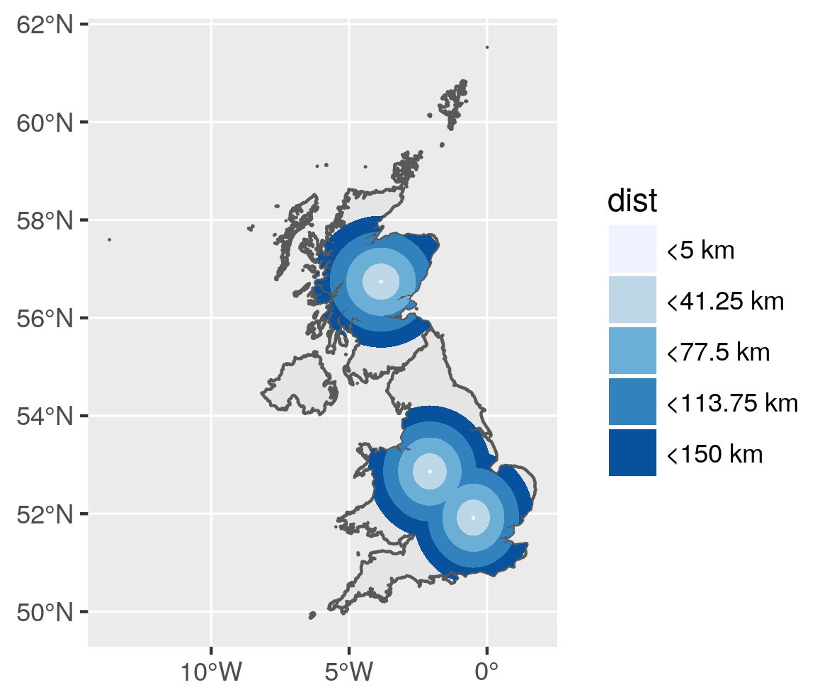
Remove areas in the sea
If you want to find proximity area on terrestrial parts only, we need to remove buffer areas that are in the sea. Intersection is computed between multipolygons with the same projection. I previously realize an union of the UK map.
# Remove part of polygons in the sea
# Union and projection of UK map
GBR_sf_merc <- st_transform(st_union(GBR_sf), 27700)
pts_holes_uk <- st_intersection(pts_holes_tot,
                              GBR_sf_merc)

ggplot() +
  geom_sf(data = GBR_sf) +
  geom_sf(data = pts_holes_uk,
          aes(fill = dist),
          colour = NA) +
  scale_fill_brewer(direction = 2)
And here is the final proximity map using sf, ggplot2 and a few other libraries...
![Proximity map]()

rgeosfunctiongBuffer()to do this. This documentation gives a good example: nickeubank.com/wp-content/uploads/2015/10/… – Sokol