Row number and partition in Excel

Question

I have data in excel such as:

ID        | Fee
123456789 | 100
987654321 | 100
987654321 | 75
987654321 | 50

I need to calculate a fee reduction for the items that are not the max price. The spreadsheet is sorted by ID, then Fee in the fashion needed. What I do not know how to do is use a similar row_number() over(partition by) in excel that I would normally do in SQL

Desired output would be

ID        | Fee   | rn
123456789 | 100   | 1
987654321 | 100   | 1
987654321 | 75    | 2
987654321 | 50    | 3

Lutenist

@pnuts, ROW_NUMBER() OVER (PARTITION BY id ORDER BY fee DESC) is a SQL Window Function. It's essentially establishing a counter, starting at 1, for each distinct ID and incrementing it for each fee, sorted descending. If ROW_NUMBER() comes up against duplicate fee's for the ID, it will continue to increment so the row_number for that ID is distinct. – Alwyn

My data looks like it does in the four sample records, the sql would really be something like row_number() over(parition by id order by fee desc), but since the data lives in an excel woorksheet the sql statement is not valid – Lutenist

Answer 1

There's probably a more complex formula one could just throw at the data without having to monkey with the data, but I think this may be an easier solution:

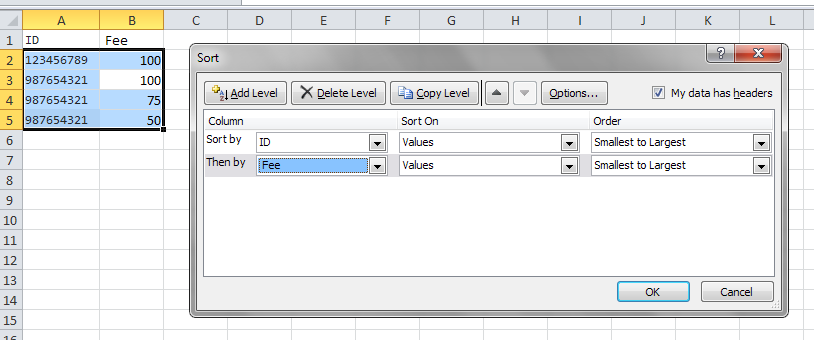
1. Sort the data by ID (smallest to largest) and Fee (Smallest to largest)

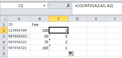
2. Use formula =Countif(A2:A5, A2) to count how many times the same id appears in the data for the current cell and every cell below it. Copying this down to fill out the missing column.

Alwyn

What I ended up doing was the following, in a separate column I did =IF(B2=B3,1,0) then in the adjacent column I did =IF(B2=B1,N1+O1,1), it only works because everything is sorted in the order I need – Lutenist

@pnuts that gives 1 the whole way down – Lutenist

@Alwyn I accepted because that will work with some possible extra sort – Lutenist

@Lutenist I ended up using your solution in your comment with an extra sort. – Clyster

Answer 2

This formula will do the job:

=COUNTIF($A$2:INDIRECT("A"&ROW(A2)),A2)

There is no need for sorting the data and you won't fall out of the range.

ROW() is used to make the range dynamic, so if we drag the formula down, ROW() will always give us ending point:

Phonology

Why would Row(A2) be different than just 2? – Tarantella

try to highlight the keywords and be clear with the format it will help to reach out your answer for others. how to answer – Scoles

@Dominique, if there was 2 instead of ROW() it would not make the range expandable. The whole idea here is to have "moving" range while progressing with the formula. – Phonology

Answer 3

you can use =COUNTIF($A$2:A2,A2); note that only the first $A$2 will not move.

Economically

Answer 4

1. Arrange everything in column A (in any order).
2. In B1 type this : =IF(A1=A2, (B2+1),1), extent this over the entire column B.

Eckhardt

Answer 5

For anyone who needs more performance, you can adjust the above query slightly to work better on large data sets.

Step one is count the maximum number of entries of a specific value in the column you wish to partition by. I did this with a pivot table.

For example, '987654321' shows up 3 times. With that information you can now limit the number of rows which the countif statement is applied to.

Then sort your data on column A. And use the below formula.

=COUNTIF(A2:INDIRECT("A"&ROW(A2)+3),A2)

This creates a rolling window for your countif function to apply too.

Lenee