How to interpret Singular Value Decomposition results (Python 3)?

Question

I'm trying to learn how to reduce dimensionality in datasets. I came across some tutorials on Principle Component Analysis and Singular Value Decomposition. I understand that it takes the dimension of greatest variance and sequentially collapses dimensions of the next highest variance (overly simplified).

I'm confused on how to interpret the output matrices. I looked at the documentation but it wasn't much help. I followed some tutorials and was not too sure what the resulting matrices were exactly. I provided some code to get a feel for the distribution of each variable in the dataset (sklearn.datasets) .

My initial input array is a (n x m) matrix of n samples and m attributes. I could do a common PCA plot of PC1 vs. PC2 but how do I know which dimensions each PC represents?

Sorry if this is a basic question. A lot of the resources are very math heavy which I'm fine with but a more intuitive answer would be useful. No where I've seen talks about how to interpret the output in terms of the original labeled data.

I'm open to using sklearn's decomposition.PCA

#Singular Value Decomposition
U, s, V = np.linalg.svd(X, full_matrices=True)
print(U.shape, s.shape, V.shape, sep="\n")
(442, 442)
(10,)
(10, 10)

Sheppard

You can refer to this pdf and stackoverflow answer for getting an intuition. I also read them few days back and they were like Bible for me. cs.otago.ac.nz/cosc453/student_tutorials/… – Melleta

stats.stackexchange.com/questions/2691/… – Melleta

Jonathan Shlens' PCA tutorial is one of the best. – Wayless

Answer 1

As you stated above matrix M can decomposed as product ot 3 matrices: U * S * V^*. Geometrical sense is next: any transformation could be deemed as a sequence of rotation (V ^* ), scaling (S) and rotation again(U). Here's good description and animation.

What's important for us? Matrix S is diagonal - all its values lying off the main diagonal are 0.

Like:

np.diag(s)

array([[ 2.00604441,  0.        ,  0.        ,  0.        ,  0.        ,         0.        ,  0.        ,  0.        ,  0.        ,  0.        ],
       [ 0.        ,  1.22160478,  0.        ,  0.        ,  0.        ,         0.        ,  0.        ,  0.        ,  0.        ,  0.        ],
       [ 0.        ,  0.        ,  1.09816315,  0.        ,  0.        ,         0.        ,  0.        ,  0.        ,  0.        ,  0.        ],
       [ 0.        ,  0.        ,  0.        ,  0.97748473,  0.        ,         0.        ,  0.        ,  0.        ,  0.        ,  0.        ],
       [ 0.        ,  0.        ,  0.        ,  0.        ,  0.81374786,         0.        ,  0.        ,  0.        ,  0.        ,  0.        ],
       [ 0.        ,  0.        ,  0.        ,  0.        ,  0.        ,         0.77634993,  0.        ,  0.        ,  0.        ,  0.        ],
       [ 0.        ,  0.        ,  0.        ,  0.        ,  0.        ,         0.        ,  0.73250287,  0.        ,  0.        ,  0.        ],
       [ 0.        ,  0.        ,  0.        ,  0.        ,  0.        ,         0.        ,  0.        ,  0.65854628,  0.        ,  0.        ],
       [ 0.        ,  0.        ,  0.        ,  0.        ,  0.        ,         0.        ,  0.        ,  0.        ,  0.27985695,  0.        ],
       [ 0.        ,  0.        ,  0.        ,  0.        ,  0.        ,         0.        ,  0.        ,  0.        ,  0.        ,  0.09252313]])

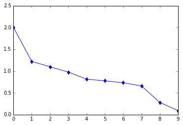
Geometrically - each value is a scaling factor along particular axis. For our purposes (Classification and Regression) these values show impact of particular axis to the overall result.

As you may see these values are decreasing from 2.0 to 0.093. One of the most important applications - easy Low-rank matrix approximation with given precision. If you do not need an ultra-precise decomposition (it is true for ML issues) you may throw off lowest values and keep only important. In such a way you may step-by-step refine your solution: estimate quality with test set, throw off least values and repeat. As a result you obtain easy and robust solution.

Here good candidates to be shrinked are 8 and 9, then 5-7, and as a last option you may approximate model to only one value - first.

Hipster

Where are the eigenvectors for The covariant matrix ? – Sheppard

Are they the columns of U or V ? Thanks for your answer btw is there a way to know which dimensions of the original dataset are represented by the eigenvectors ? – Sheppard

The columns o fU and V are left-singular vectors and right-singular vectors of M, respectively. More details here en.wikipedia.org/wiki/… – Hipster

To find covariance and which dimensions of original data set are the most valuable you may use this thing: scikit-learn.org/stable/modules/generated/… There's an attribute: explained_variance_ratio_ : array, [n_components] Percentage of variance explained by each of the selected components. If n_components is not set then all components are stored and the sum of explained variances is equal to 1.0 – Hipster