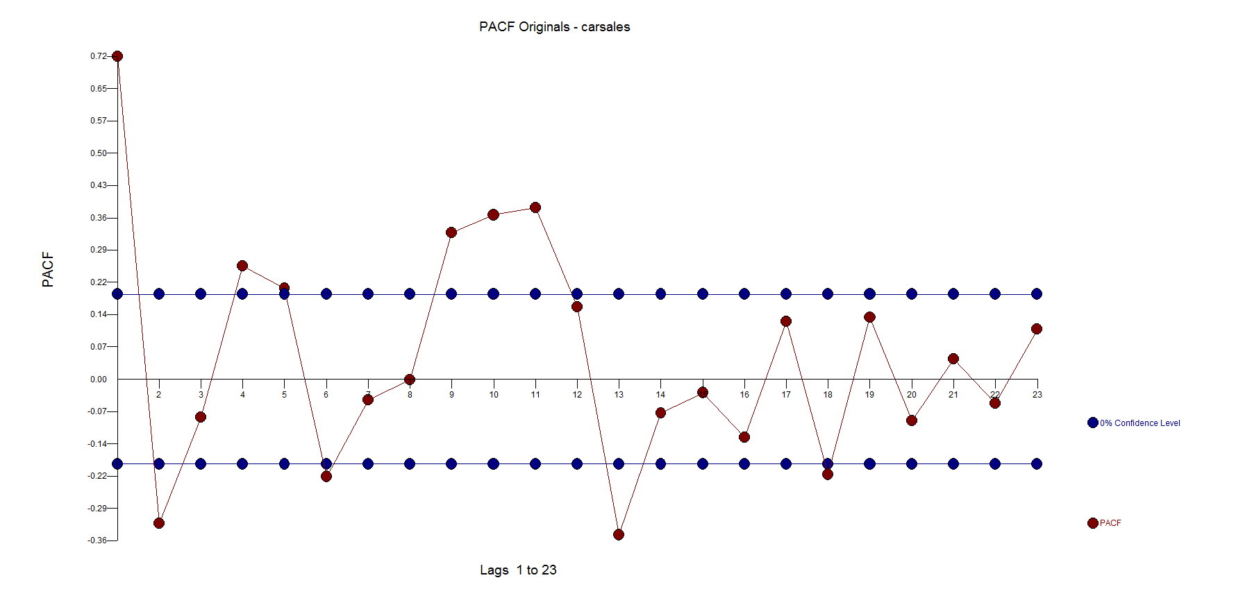
How to invert differencing in a Python statsmodels ARIMA forecast?

I'm trying to wrap my head around ARIMA forecasting using Python and Statsmodels. Specifically, for the ARIMA algorithm to work, the data needs to be made stationary via differencing (or similar method). The question is: How does one invert the differencing after the residual forecast has been made to get back to a forecast including the trend and seasonality that was differenced out?

(I saw a similar question here but alas, no answers have been posted.)

Here's what I've done so far (based on the example in the last chapter of Mastering Python Data Analysis, Magnus Vilhelm Persson; Luiz Felipe Martins). The data comes from DataMarket.

%matplotlib inline
import matplotlib.pyplot as plt
import pandas as pd
from statsmodels import tsa 
from statsmodels.tsa import stattools as stt 
from statsmodels.tsa.seasonal import seasonal_decompose
from statsmodels.tsa.arima_model import ARIMA 

def is_stationary(df, maxlag=15, autolag=None, regression='ct'): 
    """Test if df is stationary using Augmented 
    Dickey Fuller""" 

    adf_test = stt.adfuller(df,maxlag=maxlag, autolag=autolag, regression=regression) 
    adf = adf_test[0]
    cv_5 = adf_test[4]["5%"]

    result = adf < cv_5    
    return result

def d_param(df, max_lag=12):
    d = 0
    for i in range(1, max_lag):
        if is_stationary(df.diff(i).dropna()):
            d = i
            break;
    return d

def ARMA_params(df):
    p, q = tsa.stattools.arma_order_select_ic(df.dropna(),ic='aic').aic_min_order
    return p, q

# read data
carsales = pd.read_csv('data/monthly-car-sales-in-quebec-1960.csv', 
                   parse_dates=['Month'],  
                   index_col='Month',  
                   date_parser=lambda d:pd.datetime.strptime(d, '%Y-%m'))
carsales = carsales.iloc[:,0] 

# get components
carsales_decomp = seasonal_decompose(carsales, freq=12)
residuals = carsales - carsales_decomp.seasonal - carsales_decomp.trend 
residuals = residuals.dropna()

# fit model
d = d_param(carsales, max_lag=12)
p, q = ARMA_params(residuals)
model = ARIMA(residuals, order=(p, d, q)) 
model_fit = model.fit() 

# plot prediction
model_fit.plot_predict(start='1961-12-01', end='1970-01-01', alpha=0.10) 
plt.legend(loc='upper left') 
plt.xlabel('Year') 
plt.ylabel('Sales')
plt.title('Residuals 1960-1970')
print(arimares.aic, arimares.bic)

The resulting plot is satisfying, but doesn't include the trend, seasonality info. How do I invert the differencing to recapture the trend/seasonality? Residual plot

Recommended topics

Hot tags