Gaussian Process Posterior (Python)

Question

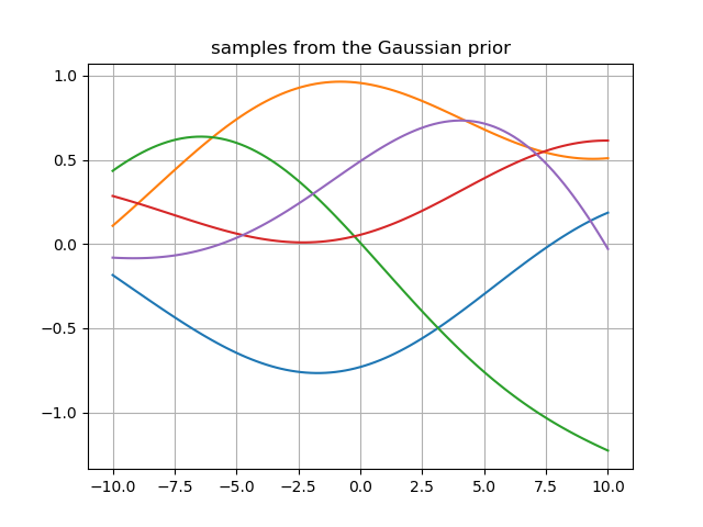
I have created and sampled a jointly Gaussian prior with mean=0 using the code below:

import numpy as np
import matplotlib.pyplot as plt 
from math import pi 
from scipy.spatial.distance import cdist
import scipy.stats as sts

x_prior = np.linspace(-10,10,101)
x_prior = x_prior.reshape(-1,1)
mu = np.zeros(x_prior.shape)

#defining the Kernel for the covariance function

def sec(a,b, length_scale , sigma) : 
    K = sigma * np.exp(-1/(2*length_scale) * cdist(a,b)**2)
    return K 

#defining the Gaussian Process prior

def GP(a , b, mu , kernel , length_scale, sigma , samples ) :
    f = np.random.multivariate_normal(mu.flatten(), kernel(a ,b , length_scale , sigma ) , samples)
    return f

prior = GP(x_prior ,x_prior, mu , sec , 100, 1 , 5)

plt.figure()
plt.grid()
plt.title('samples from the Gaussian prior')
plt.plot(x_prior , prior.T)
plt.show()

Then, when adding in some 'observed' data, I wish to compute the posterior over these points but this is where I become stuck.

Here's my code for introducing new data:

x_train = np.array([-10,-8,5,-1,2])
x_train = x_train.reshape(-1,1)
def straight_line(m , x , c):
    y = 5*x + c
    return y
ytrain = straight_line(5 , x_train , 0)

It's my understanding that you calculate a conditional distribution over the new data given the prior and new x values associated with the observed data.

Do you then wish to update the multivariate prior to become the posterior by performing some sort of change to the mean values to include the new y values?

I have used the following resources to try and attempt this:

http://katbailey.github.io/post/gaussian-processes-for-dummies/ https://www.robots.ox.ac.uk/~mebden/reports/GPtutorial.pdf

but I'm really trying to understand what happens at each stage, and why, so that when I get a posterior (which I can't do) I know exactly how I got there.

Here's some solutions I've been trying to implement but so far no avail:

K_train = sec(x_train , x_train , 1,1)
K_prior = sec(x_prior , x_prior , 1,1)
K_pt =  sec(x_prior , x_train , 1,1)
K_tp = sec(x_train , x_prior ,  1,1)  ## = k_tp transpose
prior = sts.multivariate_normal(mu.flatten(), K_prior) 
#mean_test = np.dot(K_p , np.linalg.inv(K_prior))
mean_function = np.dot(np.dot(K_tp ,np.linalg.inv(K_prior).T) , prior )
covariance_function = K_train - np.dot(np.dot(K_tp ,np.linalg.inv(K_prior).T) , K_pt) 

Mola

Answer 1

Just for additional follow-up. I have written my code into a Juypiter format here:

https://github.com/SpaceMeerkat/Scariff

with associated read-through material here:

https://spacemeerkat.wordpress.com/

Just in case anyone wanted to work through this kind of material and became stuck like I did.

Mola

Answer 2

Just an update for anyone who looked at this. I found the solution reading this paper:

https://arxiv.org/pdf/1711.10834.pdf

and the following code:

mean_function = np.dot(np.dot(K_pt ,np.linalg.inv(K_train)), ytrain) 

covariance_function = K_prior - np.dot(np.dot(K_pt ,np.linalg.inv(K_train)) , K_tp) 

f = np.random.multivariate_normal(mean_function[:,0],covariance_function , 100)

where f is the posterior joint Gaussian from which you sample from

Mola

Answer 3

The prediction (Krigging) for a new point x* with Gaussian Process, having observed the data x(1:N), y(1:N) has the following form:

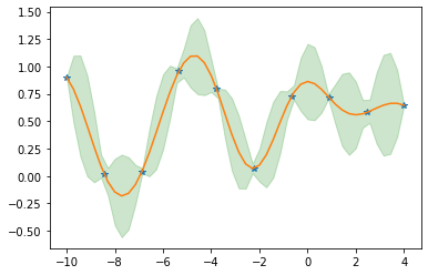
The below code shows the implementation of the above Bayesian update equations to compute the posterior given the prior and the observed data (here blue stars represent the training datapoints and red line the corresponding predictions with GP and the green band being the confidence interval):

x_train = np.linspace(-10, 4, 10).reshape(-1,1)
y_train = np.random.random(10)
x_p = np.linspace(-10, 4, 50).reshape(-1,1) 
K_train = kernel(x_train, x_train, length_scale=2, sigma=1)
K_pt = kernel(x_p, x_train, length_scale=2, sigma=1)
K_tp = kernel(x_train, x_p, length_scale=2, sigma=1)
K_prior = kernel(x_p, x_p, length_scale=2, sigma=1)
# compute posterior
mean_function = np.dot(np.dot(K_pt ,np.linalg.inv(K_train)), y_train) 
covariance_function = K_prior - np.dot(np.dot(K_pt ,np.linalg.inv(K_train)) , K_tp) 
plt.plot(x_train, y_train, '*')
plt.plot(x_p, mean_function)
plt.fill_between(x_p.ravel(), mean_function-3*np.sqrt(np.diag(covariance_function)), mean_function+3*np.sqrt(np.diag(covariance_function)), color='g', alpha=.2)

The predictive posterior distribution is shown in the next figure:

Colcothar