conditional sampling from multivariate kernel density estimate in python

Question

One can create a multivariate kernel density estimate (KDE) with scikitlearn (https://scikit-learn.org/stable/modules/generated/sklearn.neighbors.KernelDensity.html#sklearn.neighbors.KernelDensity) and scipy (https://docs.scipy.org/doc/scipy/reference/generated/scipy.stats.gaussian_kde.html)

Both allow for random sampling from the estimated distribution. Is there a way to do conditional sampling in either of the two libraries (or any other library)? In the 2-variable (x,y) case this would mean sample from P(x|y) (or P(y|x)), thus from a cross-section of the probability function (and that cross-section has to be rescaled to unit area under its curve).

x = np.random.random(100)
y =np.random.random(100)
kde = stats.gaussian_kde([x,y])
# sampling from the whole pdf:
kde.resample()

I am looking for something like

# sampling y, conditional on x
kde.sample_conditional(x=1.5) #does not exist

Dropwort

Have you solved this? – Loni

also interested in this. – Klaus

any development? – Several

Check my answer – Several

Answer 1

This function samples conditionally one column based on all other columns.

def conditional_sample(kde, training_data, columns, values, samples = 100):
    if len(values) - len(columns) != 0:
        raise ValueError("length of columns and values should be equal")
    if training_data.shape[1] - len(columns) != 1:
        raise ValueError(f'Expected {training_data.shape[1] - 1} columns/values but {len(columns)} have be given')  
    cols_values_dict = dict(zip(columns, values))
    
    #create array to sample from
    steps = 10000  
    X_test = np.zeros((steps,training_data.shape[1]))
    for i in range(training_data.shape[1]):
        col_data = training_data.iloc[:, i]
        X_test[:, i] = np.linspace(col_data.min(),col_data.max(),steps)
    for col in columns: 
        idx_col_training_data = list(training_data.columns).index(col)
        idx_in_values_list = list(cols_values_dict.keys()).index(col)
        X_test[:, idx_col_training_data] = values[idx_in_values_list] 
        
    #compute probability of each sample
    prob_dist = np.exp(kde.score_samples(X_test))/np.exp(kde.score_samples(X_test)).sum()
    
    #sample using np.random.choice
    return X_test[np.random.choice(range(len(prob_dist)), p=prob_dist, size = (samples))]

Several

nice workaround for part of the problem, but not for everything. If I understand it correctly, it works with probing the KDE with a discrete grid, which will introduce errors. Also, a KDE can actually extrapolate beyond the smallest and largest training point along an axis, which this method wont be able to do. – Dropwort

Indeed for more efficient conditional sampling, we need to construct the pdf i think. Sadly no implementation of pdf in sklearn.kde and no sampling implementation of sampling in statsmodels.kde – Several

Answer 2

This function works for use cases with only 1-dimensional conditions. It's built in a way that the condition doesn't need to be fulfilled exactly, but with some tolerance.

from scipy import stats
import numpy as np

x = np.random.random(1000)
y = np.random.random(1000)
kde = stats.gaussian_kde([x,y])

def conditional_sample(kde, condition, precision = 0.5,  sample_size = 1000):

    block_size = int(sample_size / (2 * precision / 100))
    sample = kde.resample(block_size)

    lower_limit = np.percentile(sample[-1], stats.percentileofscore(sample[-1], condition) - precision)
    upper_limit = np.percentile(sample[-1], stats.percentileofscore(sample[-1], condition) + precision)

    conditional_sample = sample[:, (upper_limit > sample[-1]) * (sample[-1] > lower_limit)]

    return conditional_sample[0:-1]

conditional_sample(kde=kde, condition=0.6)

Not a universal solution but works well for my use case.

Transmittal

Your answer could be improved with additional supporting information. Please edit to add further details, such as citations or documentation, so that others can confirm that your answer is correct. You can find more information on how to write good answers in the help center. – Mashhad

Answer 3

statsmodels KDEMultivariateConditional implements conditional KDEs. It can compute conditional pdf and cdf. While it has no built-in sampling method, the generic approach of inverse transform sampling can be used (see this answer). Note that this is probably not the most efficient way to do this. Here is an example in 2D:

import numpy as np
from statsmodels.nonparametric.kernel_density import KDEMultivariateConditional
from pylab import plt
from scipy.optimize import brentq

# generate data with some autocorrelation to make it interesting
x_train = np.random.normal(size=1000)
y_train = x_train + np.random.normal(size=1000)

# train conditional KDE
kde = KDEMultivariateConditional(endog=y_train, exog=x_train, dep_type='c', 
                                 indep_type='c', bw='normal_reference')

def cdf_conditional(x, y_target):
    # cdf of kde conditional on x, evaluated at y_target
    return kde.cdf(np.array(y_target).reshape((-1,1)), np.array(x).reshape((-1,1)))

# inverse-transform-sampling
def sample_conditional_single(x):
    # sample conditional on x
    u = np.random.random()
    # 1-d root-finding
    def func(y):
        return cdf_conditional(x, y)- u
    sample_y = brentq(func, -99999999, 99999999)  # read brentq-docs about these constants
                                                # constants need to be sign-changing for the function
    return sample_y

def sample_conditional(x, n):
    return np.array([sample_conditional_single(x) for _ in range(n)])


# now sample at 2 different x values
x1 = 0
x2 = 2
samples1 = sample_conditional(x1, 100)
samples2 = sample_conditional(x2, 100)

plt.figure()
plt.scatter(x_train, y_train)
plt.xlabel('x')
plt.ylabel('y')
plt.title("training data")
plt.figure()
plt.scatter(np.repeat(np.array(x1), len(samples1)), samples1)
plt.scatter(np.repeat(np.array(x2), len(samples2)), samples2)
plt.xlabel('x')
plt.ylabel('y')
plt.title('sampled conditionally')

Dropwort

Answer 4

I also searched without success for multivariate KDE conditional sampling functionality, so I wrote a subclass of scipy.stats.gaussian_kde() with a conditional_resample() method: https://pypi.org/project/kdetools/

You can conditionally sample from any subset of the variables, do vectorised sampling for multiple conditioning vectors, as well as doing bandwidth selection using k-fold CV using different kinds of bandwidth matrices. The code is still somewhat a work in progress, e.g. need to add some tests, and I can't quite replicate statsmodels/R multivariate bandwidth selection results. Happy for people to stress-test it and give feedback.

As a toy example, I created a 3-component Gaussian mixture, sampled from it and fit KDEs using a few different bandwidth approaches:

import numpy as np
import matplotlib.pyplot as plt
import kdetools as kt

# Generate toy 2D mixture of 3 Gaussians, all centred on 0 in the x-direction
np.random.seed(0)
N = 200
X = np.vstack([np.random.multivariate_normal([0,0],[[1.5,-0.5],[-0.5,1]], size=N),
               np.random.multivariate_normal([0,3],[[1,0.5],[0.5,1.5]], size=N),
               np.random.multivariate_normal([0,6],[[2,1],[1,1.5]], size=N)])

# Define the mixture pdf
def zz_pdf_func(X):
    zz_pdf1 = st.multivariate_normal([0,0],[[1.5,-0.5],[-0.5,1]])
    zz_pdf2 = st.multivariate_normal([0,3],[[1,0.5],[0.5,1.5]])
    zz_pdf3 = st.multivariate_normal([0,6],[[2,1],[1,1.5]])
    return (zz_pdf1.pdf(X)+zz_pdf2.pdf(X)+zz_pdf3.pdf(X))/3

# Fit KDEs using different bandwidth types
kde1 = kt.gaussian_kde(X.T)
kde2 = kt.gaussian_kde(X.T); kde2.set_bandwidth('cv', bw_type='equal')
kde3 = kt.gaussian_kde(X.T); kde3.set_bandwidth('cv', bw_type='diagonal')
kde4 = kt.gaussian_kde(X.T); kde4.set_bandwidth('cv', bw_type='covariance')

# Plot 2D KDEs and overlay contours of true distribution in red:
xx, yy = np.meshgrid(np.linspace(-5, 5, 1000), np.linspace(-3, 10, 1000)) 
zz_pdf = zz_pdf_func(np.stack([xx.ravel(), yy.ravel()]).T).reshape(xx.shape)
fig, ((ax1, ax2), (ax3, ax4)) = plt.subplots(2, 2, figsize=(10,10))
zz_kde1 = kde1.pdf(np.stack([xx.ravel(), yy.ravel()])).reshape(xx.shape)
zz_kde2 = kde2.pdf(np.stack([xx.ravel(), yy.ravel()])).reshape(xx.shape)
zz_kde3 = kde3.pdf(np.stack([xx.ravel(), yy.ravel()])).reshape(xx.shape)
zz_kde4 = kde4.pdf(np.stack([xx.ravel(), yy.ravel()])).reshape(xx.shape)

ax1.contourf(xx, yy, zz_kde1, alpha=0.95)
ax1.contour(xx, yy, zz_pdf, colors='r', linewidths=0.25)
ax1.scatter(X[:,0], X[:,1], s=1)
ax1.set_title('Standard - scaled full covariance')

ax2.contourf(xx, yy, zz_kde2, alpha=0.95)
ax2.contour(xx, yy, zz_pdf, colors='r', linewidths=0.25)
ax2.scatter(X[:,0], X[:,1], s=1)
ax2.set_title('CV - spherical covariance matrix')

ax3.contourf(xx, yy, zz_kde3, alpha=0.95)
ax3.contour(xx, yy, zz_pdf, colors='r', linewidths=0.25)
ax3.scatter(X[:,0], X[:,1], s=1)
ax3.set_title('CV - diagonal covariance matrix')

ax4.contourf(xx, yy, zz_kde4, alpha=0.95)
ax4.contour(xx, yy, zz_pdf, colors='r', linewidths=0.25)
ax4.scatter(X[:,0], X[:,1], s=1)
ax4.set_title('CV - scaled full covariance matrix');

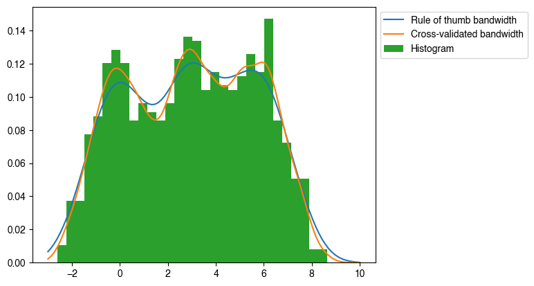
Having generated the KDE, I took conditional samples of y|x=0 and generated another histogram/KDE:

np.random.seed(42)
y = kde3.conditional_resample(1000, x_cond=np.array([0]), dims_cond=[0]).ravel()
kde1d = kt.gaussian_kde(y)
xs = np.linspace(-3, 10, 100)
plt.plot(xs, kde1d.pdf(xs), label='Rule of thumb bandwidth')

# Update the bandwidth
kde1d.set_bandwidth(bw_method='cv', bw_type='equal')
xs = np.linspace(-3, 10, 100)
plt.plot(xs, kde1d.pdf(xs), label='Cross-validated bandwidth')

plt.hist(y, bins=30, density=True, label='Histogram')

plt.legend(bbox_to_anchor=(1,1));

Arctic