How to properly join data and geometry using ggmap

Question

An image is worth a thousand words:

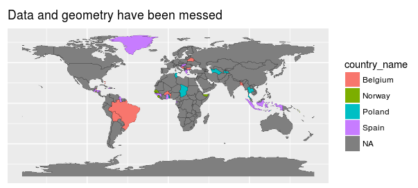
Observed behaviour: As can be seen from the image above, countries' names do not match with their actual geometries.

Expected behaviour: I would like to properly join a data frame with its geometry and display the result in ggmap.

I've previously joined different data frames, but things get wrong by the fact that apparently ggmap needs to "fortify" (actually I don't know what really means) data frame in order to display results.

This is what I've done so far:

library(rgdal)
library(dplyr)
library(broom)
library(ggmap)

# Load GeoJSON file with countries.
countries = readOGR(dsn = "https://gist.githubusercontent.com/ccamara/fc26d8bb7e777488b446fbaad1e6ea63/raw/a6f69b6c3b4a75b02858e966b9d36c85982cbd32/countries.geojson")

# Load dataframe.
df = read.csv("https://gist.githubusercontent.com/ccamara/fc26d8bb7e777488b446fbaad1e6ea63/raw/a6f69b6c3b4a75b02858e966b9d36c85982cbd32/sample-dataframe.csv")

# Join geometry with dataframe.
countries$iso_a2 = as.factor(countries$iso_a2)
countries@data = left_join(countries@data, df, by = c('iso_a2' = 'country_code'))

# Convert to dataframe so it can be used by ggmap.
countries.t = tidy(countries)

# Here's where the problem starts, as by doing so, data has been lost!

# Recover attributes' table that was destroyed after using broom::tidy.
countries@data$id = rownames(countries@data) # Adding a new id variable.
countries.t = left_join(countries.t, countries@data, by = "id")

ggplot(data = countries.t,
       aes(long, lat, fill = country_name, group = group)) +
  geom_polygon() +
  geom_path(colour="black", lwd=0.05) + # polygon borders
  coord_equal() +
  ggtitle("Data and geometry have been messed!") +
  theme(axis.text = element_blank(), # change the theme options
        axis.title = element_blank(), # remove axis titles
        axis.ticks = element_blank()) # remove axis ticks

Spurlock

Answer 1

There is a reason for the messed up behaviour.

countries starts out as a large SpatialPolygonsDataFrame with 177 elements (and correspondingly 177 rows in countries@data). When you perform left_join on countries@data and df, the number of elements in countries isn't affected, but the number of rows in countries@data grows to 210.

Fortifying countries using broom::tidy converts countries, with its 177 elements, into a data frame with id running from 0 to 176. (I'm not sure why it's zero-indexed, but I usually prefer to specify the regions explicitly anyway).

Adding id to countries@data based on rownames(countries@data), on the other hand, results in id values running from 1 to 210, since that's the number of rows in countries@data after the earlier join with df. Consequently, everything is out of sync.

Try the following instead:

# (we start out right after loading countries & df)

# no need to join geometry with df first

# convert countries to data frame, specifying the regions explicitly
# (note I'm using the name column rather than the iso_a2 column from countries@data;
# this is because there are some repeat -99 values in iso_a2, and we want
# one-to-one matching.)
countries.t = tidy(countries, region = "name")

# join with the original file's data
countries.t = left_join(countries.t, countries@data, by = c("id" = "name"))

# join with df
countries.t = left_join(countries.t, df, by = c("iso_a2" = "country_code"))

# no change to the plot's code, except for ggtitle
ggplot(data = countries.t,
       aes(long, lat, fill = country_name, group = group)) +
  geom_polygon() +
  geom_path(colour="black", lwd = 0.05) +
  coord_equal() +
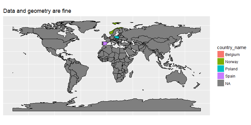
  ggtitle("Data and geometry are fine") +
  theme(axis.text = element_blank(),
        axis.title = element_blank(),
        axis.ticks = element_blank())

p.s. You don't actually need the ggmap package for this. Just the ggplot2 package that it loads.

Hick

Thank you for such a great explanation! Your solution works great! There's something I do not understand though (even after having checked ?broom::tidy): It seems to me that the statement countries.t = tidy(countries, region = "name") is key in your answer, but I do not understand what region="name" exactly does, despite I have observed notable differences in the output if I just type countries.t = tidy(countries) – Spurlock

And thanks for pointing out that ggmap is not needed for these matters. I wanted to do some more things, though, but everything relies on fixing this issue ;) – Spurlock

@Spurlock As per ?broom::sp_tidy.SpatialPolygonsDataFrame, the region argument specifies the name of the variable from countries@data to be used to split up regions. – Hick

If region is unspecified, each row of countries@data is treated as a separate region, and countries.t$id takes on the values 0-176 (based on row number of countries@data - 1). If you specify region = "name", each group of rows with a different countries@data$name value is treated as a separate region, and countries.t$id takes on the values of country names. This allows us to join countries.t with other data frames by country name, rather than depend on matching the original row numbers. – Hick

Thanks for the explanation, I could not find that information (or understand it) in the command's built-in help. Much clearer now. – Spurlock

Answer 2

While your work is a reasonable approach - I would like to rethink your design, mainly because of two simple reasons:

1) while GeoJSON is the future, R still heavily relies on the sp package and its correspondent sp* objects - very soon you wish you had switched early on. It`s just about the packages and most of them (if not all) rely on sp* objects.

2) ggplot has great plotting capabilities combined with ggmap - but its still quite limited compared to sp* in combination with leaflet for R etc.

probably the fastest way to go is simple as:

library(sp)
library(dplyr)
library(geojsonio)
library(dplyr)
library(tmap)

#get sp* object instead of geojson
countries <- geojsonio::geojson_read("foo.geojson",what = "sp")

#match sp* object with your data.frame
countries@data <- dplyr::left_join(countries@data, your_df, by = 
c("identifier_1" = "identifier_2"))

#creates a fast and nice looking plot / lots of configuration available
p1 <- tm_shape(countries) +
      tm_polygons() 
p1

#optional interactive leaflet plot
tmap_leaflet(p1)

It is written out of my head / bear with me if there are minor issues.

It is a different approach but its at least in my eyes a faster and more concise approach in R right now (hopefully geojson will receive more support in the future).

Jodijodie

Thank you for your answer. I am currently testing options and tmap is indeed a good choice. In fact it was my first one, but I ended up with this error: #46298566 (I think I am doing the same approach as you did) and that's why I ended trying ggmap (that and the lack of option of adding a map's title!). By the way, there's something I do not understand about your answer: what do you mean by sp* objects? are there some R-object types? – Spurlock

read the documentation of the "sp" package - from start to nearly end. It is easy to read and will give you a proper overview how to deal with spatial data. Afterwards everything seems half as hard as it used to be. – Jodijodie