What is the time complexity of numpy.linalg.det?

The documentation for numpy.linalg.det states that

The determinant is computed via LU factorization using the LAPACK routine z/dgetrf.

I ran the following run time tests and fit polynomials of degrees 2, 3, and 4 because that covers the least worst options in this table. That table also mentions that an LU decomposition approach takes $O(n^3)$ time, but then the theoretical complexity of LU decomposition given here is $O(n^{2.376})$. Naturally the choice of algorithm matters, but I am not sure what available time complexities I should expect from numpy.linalg.det.

from timeit import timeit

import matplotlib.pyplot as plt
import numpy as np
from sklearn.linear_model import LinearRegression
from sklearn.preprocessing import PolynomialFeatures


sizes = np.arange(1,10001, 100)
times = []

for size in sizes:
    A = np.ones((size, size))
    time = timeit('np.linalg.det(A)', globals={'np':np, 'A':A}, number=1)
    times.append(time)
    print(size, time)

sizes = sizes.reshape(-1,1)
times = np.array(times).reshape(-1,1)

quad_sizes = PolynomialFeatures(degree=2).fit_transform(sizes)
quad_times = LinearRegression().fit(quad_sizes, times).predict(quad_sizes)
cubic_sizes = PolynomialFeatures(degree=3).fit_transform(sizes)
cubic_times = LinearRegression().fit(cubic_sizes, times).predict(cubic_sizes)
quartic_sizes = PolynomialFeatures(degree=4).fit_transform(sizes)
quartic_times = LinearRegression().fit(quartic_sizes, times).predict(quartic_sizes)

plt.scatter(sizes, times, label='Data', color='k', alpha=0.5)
plt.plot(sizes, quad_times, label='Quadratic', color='r')
plt.plot(sizes, cubic_times, label='Cubic', color='g')
plt.plot(sizes, quartic_times, label='Quartic', color='b')
plt.xlabel('Matrix Dimension n')
plt.ylabel('Time (seconds)')
plt.legend()
plt.show()

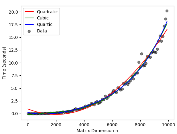
The output of the above is given as the following plot.

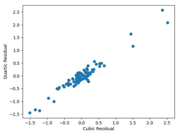
Since none of the available complexities get down to quadratic time, I am unsurprising that visually the quadratic model had the worst fit. Both the cubic and quartic models had excellent visual fit, and unsurprisingly their residuals are closely correlated.

Some related questions exist, but they do not have an answer for this specific implementation.

Since this implementation is used by a lot of Python programmers world-wide, it may benefit the understanding of a lot of people if an answer was tracked down.

TL;DR: it is between O(n^2.81) and O(n^3) regarding the target BLAS implementation.

Indeed, Numpy uses a LU decomposition (in the log space). The actual implementation can be found here. It indeed uses the sgetrf/dgetrf primitive of LAPACK. Multiple libraries provides such a libraries. The most famous is the one of NetLib though it is not the fastest. The Intel MKL is an example of library providing a fast implementation. Fast LU decomposition algorithms use tiling methods so to use a matrix multiplication internally. Their do that because the matrix multiplication is one of the most optimized methods linear algebra libraries (for example the MKL, BLIS, and OpenBLAS generally succeed to reach nearly optimal performance on modern processors). More generally, the complexity of the LU decomposition is the one of the matrix multiplication.

The complexity of the naive squared matrix multiplication is O(n^3). Faster algorithms exists like Strassen (running in ~O(n^2.81) time) which is often used for big matrices. The Coppersmith–Winograd algorithm achieves a significantly better complexity (~O(n^2.38)), but no linear algebra libraries actually use it since it is a galactic algorithm. Put it shortly, such algorithm is theoretically asymptotically better than others but the hidden constant make it impractical for any real-world usage. For more information about the complexity of the matrix multiplication, please read this article. Thus, in practice, the complexity of the matrix multiplication is between O(n^2.81) and O(n^3) regarding the target BLAS implementation (which is dependent of your platform and your configuration of Numpy).

Recommended topics

Hot tags