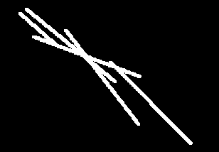
This is a great question. The right way to look at this is to integrate the error along each line segment. Instead of a simple term (y[i] - y_hat)^2 (where y_hat is the predicted value from the regression line) you should have integral((y[i](t) - y_hat)^2, t, 0, 1) where y[i](t) is parametrization of the line segment, y[i](t) = t * y[i, 1] + (1 - t)*y[i, 0] (denoting the endpoints of the i-th segment as y[i, 0] and y[i, 1]). I think you'll find that you can compute the integral exactly and therefore you'll get terms for the sum of squared errors which involve just the endpoints. I've left out some details but I think that's enough for you to work out the rest. EDIT: Error terms should be squared; I've adjusted formulas accordingly.
2ND EDIT: I worked out some formulas (using Maxima). For a regression line represented by y = alpha*x + beta, I get as the least squares estimates for alpha and beta:
alpha = (4*('sum(ll[k],k,1,n))*'sum(xx[k][2]*yy[k][2]*ll[k],k,1,n)
    +2*('sum(ll[k],k,1,n))*'sum(xx[k][1]*yy[k][2]*ll[k],k,1,n)
    +('sum(xx[k][2]*ll[k],k,1,n))*(-3*'sum(yy[k][2]*ll[k],k,1,n)
                                  -3*'sum(yy[k][1]*ll[k],k,1,n))
    +('sum(xx[k][1]*ll[k],k,1,n))*(-3*'sum(yy[k][2]*ll[k],k,1,n)
                                  -3*'sum(yy[k][1]*ll[k],k,1,n))
    +2*('sum(ll[k],k,1,n))*'sum(yy[k][1]*xx[k][2]*ll[k],k,1,n)
    +4*('sum(ll[k],k,1,n))*'sum(xx[k][1]*yy[k][1]*ll[k],k,1,n))
    /(4*('sum(ll[k],k,1,n))*'sum(xx[k][2]^2*ll[k],k,1,n)
     +4*('sum(ll[k],k,1,n))*'sum(xx[k][1]*xx[k][2]*ll[k],k,1,n)
     -3*('sum(xx[k][2]*ll[k],k,1,n))^2
     -6*('sum(xx[k][1]*ll[k],k,1,n))*'sum(xx[k][2]*ll[k],k,1,n)
     +4*('sum(ll[k],k,1,n))*'sum(xx[k][1]^2*ll[k],k,1,n)
     -3*('sum(xx[k][1]*ll[k],k,1,n))^2)

  beta = -((2*'sum(xx[k][2]*ll[k],k,1,n)+2*'sum(xx[k][1]*ll[k],k,1,n))
   *'sum(xx[k][2]*yy[k][2]*ll[k],k,1,n)
   +('sum(xx[k][2]*ll[k],k,1,n)+'sum(xx[k][1]*ll[k],k,1,n))
    *'sum(xx[k][1]*yy[k][2]*ll[k],k,1,n)
   +('sum(xx[k][2]^2*ll[k],k,1,n))*(-2*'sum(yy[k][2]*ll[k],k,1,n)
                                   -2*'sum(yy[k][1]*ll[k],k,1,n))
   +('sum(xx[k][1]*xx[k][2]*ll[k],k,1,n))
    *(-2*'sum(yy[k][2]*ll[k],k,1,n)-2*'sum(yy[k][1]*ll[k],k,1,n))
   +('sum(xx[k][1]^2*ll[k],k,1,n))*(-2*'sum(yy[k][2]*ll[k],k,1,n)
                                   -2*'sum(yy[k][1]*ll[k],k,1,n))
   +('sum(xx[k][2]*ll[k],k,1,n)+'sum(xx[k][1]*ll[k],k,1,n))
    *'sum(yy[k][1]*xx[k][2]*ll[k],k,1,n)
   +2*('sum(xx[k][1]*yy[k][1]*ll[k],k,1,n))*'sum(xx[k][2]*ll[k],k,1,n)
   +2*('sum(xx[k][1]*ll[k],k,1,n))*'sum(xx[k][1]*yy[k][1]*ll[k],k,1,n))
   /(4*('sum(ll[k],k,1,n))*'sum(xx[k][2]^2*ll[k],k,1,n)
    +4*('sum(ll[k],k,1,n))*'sum(xx[k][1]*xx[k][2]*ll[k],k,1,n)
    -3*('sum(xx[k][2]*ll[k],k,1,n))^2
    -6*('sum(xx[k][1]*ll[k],k,1,n))*'sum(xx[k][2]*ll[k],k,1,n)
    +4*('sum(ll[k],k,1,n))*'sum(xx[k][1]^2*ll[k],k,1,n)
    -3*('sum(xx[k][1]*ll[k],k,1,n))^2)
where xx and yy are lists of pairs of values, one pair for each line segment. That is, xx[k] are the x-coordinates for the endpoints of the k-th segment, yy[k] are the y-coordinates for the endpoints of the k-th segment, and ll[k] is the length sqrt((xx[k][2] - xx[k][1])^2 + (yy[k][2] - yy[k][1])^2) of the k-th segment.
Here is my program to derive those formulas. Probably there are other reasonable ways to set up this problem which yield similar but different formulas.
y_hat[k](l) := alpha * x[k](l) + beta;
x[k](l) := (1 - l/ll[k]) * xx[k][1] + l/ll[k] * xx[k][2];
y[k](l) := (1 - l/ll[k]) * yy[k][1] + l/ll[k] * yy[k][2];
e[k]:= y[k](l) - y_hat[k](l);
foo : sum (integrate (e[k]^2, l, 0, ll[k]), k, 1, n);
declare (nounify (sum), linear);
[da, db] : [diff (foo, alpha), diff (foo, beta)];
map (expand, %);
bar : solve (%, [alpha, beta]);
Here are some example data and the result I get. I postponed defining dx, dy, and ll because, since they are all constant terms, I didn't want them to be expanded in the solutions for alpha and beta.
dx[k] := xx[k][2] - xx[k][1];
dy[k] := yy[k][2] - yy[k][1];
ll[k] := sqrt (dx[k]^2 + dy[k]^2);

xx : [[1,2],[1.5,3.5],[5.5,10.5]]$
yy : [[1,2.2],[1.5,3.3],[5,12]]$

''bar, nouns, n=length(xx);
  => [[alpha = 1.133149837130799, beta = - 0.4809409869515073]]


