Three-level nested mixed-effects model

Question

I am trying to model a three-level nested linear mixed effects model in rjags (by three-level: multiple observations for multiple individuals within multiple groups). There are unique sets of individuals in the groups.

The equivalent model in lme4 would be

lmer(yN ~ x + (1 |group/indiv), data=qq)

or

lmer(yN ~ x + (1 |group) + (1|indiv), data=qq)

My question is: How do I program this model in rjags please.

---

This is my attempt at the rjags code, which compiles, and executes but the individual level random effects seem to be penalised too much - enough to suggest that it is coded incorrectly.

st <- "
model {

  for(i in 1:n){
      mu[i] <- beta[1] + b1[ind[i]] + b2[group[i]] + beta[2]* x[i] 
      y[i] ~ dnorm(mu[i], tau)
  }

  for(i in 1:2){  beta[i] ~ dnorm(0, 0.0001)  }

  tau ~ dgamma(0.01, 0.01)
  sigma <- sqrt(1/tau) 

  # hierarchical model
  for (i in 1:nInd) { b1[i] ~ dnorm(0, tau0) }
  for (i in 1:nGrp) { b2[i] ~ dnorm(0, tau1) }

  tau0 ~ dgamma(0.001, 0.001)
  sigma0 <- sqrt(1/tau0) 
  tau1 ~ dgamma(0.001, 0.001)
  sigma1 <- sqrt(1/tau1) 
}
"

And run model

library(rjags)

mod <- jags.model( textConnection(st),
                 data=list(y=qq$yN, 
                           x=qq$x, 
                           ind=qq$indiv, 
                           group=qq$group,
                           n=nrow(qq),
                           nInd=length(unique(qq$indiv)),
                           nGrp=length(unique(qq$group))),
                 n.adapt=1e6,
                 inits=list(.RNG.seed=1,
                            .RNG.name="base::Wichmann-Hill")
                )
mod <- coda.samples(mod, 
                   variable.names=c("beta","b1", "b2", "sigma", "sigma0", "sigma1"), 
                   n.iter=1e6, 
                   thin=5)

summary(mod)

qq <- structure(list(yN = c(3.51, 5.13, 5.2, 7.46, 5.64, 5.14, 6.84, 
7.19, 7.77, 6, 10.97, 9.75, 5.43, 1.11, 10.31, 5.3, 4.52, 4.62, 
3.97, 4.31, 8.2, 7.24, 6.75, 0, 7.77, 4.25, 5.29, 2.46, 4.3, 
6.67, 8.72, 7.52, 6.12, 6.02, 1.48, 4.65, 7.52, 5.88, 6.06, 5.27, 
6.04, 5.36, 7.34, 6.39, 2.84, 3.95, 8.07, 7.22, 4.78, 9.92, 5.85, 
2.75, 6.34, 2.62, 7.3, 15.45, 5, 1.52, 8.3, 6.25, 16.32, 5.67, 
8.55, 5.72, 2.8, 6.06, 1.3, 11.74, 7.02, 12.85, 6.46, 3.68, 8.48, 
0.28, 0.92), x = c(-0.63, 0.18, -0.84, 1.6, 0.33, -0.82, 0.49, 
0.74, 0.58, -0.31, 1.51, 0.39, -0.62, -2.21, 1.12, -0.04, -0.02, 
0.94, 0.82, 0.59, 0.92, 0.78, 0.07, -1.99, 0.62, -0.06, -0.16, 
-1.47, -0.48, 0.42, 1.36, -0.1, 0.39, -0.05, -1.38, -0.41, -0.39, 
-0.06, 1.1, 0.76, -0.16, -0.25, 0.7, 0.56, -0.69, -0.71, 0.36, 
0.77, -0.11, 0.88, 0.4, -0.61, 0.34, -1.13, 1.43, 1.98, -0.37, 
-1.04, 0.57, -0.14, 2.4, -0.04, 0.69, 0.03, -0.74, 0.19, -1.8, 
1.47, 0.15, 2.17, 0.48, -0.71, 0.61, -0.93, -1.25), indiv = structure(c(1L, 
1L, 1L, 1L, 1L, 2L, 2L, 2L, 2L, 2L, 3L, 3L, 3L, 3L, 3L, 4L, 4L, 
4L, 4L, 4L, 5L, 5L, 5L, 5L, 5L, 6L, 6L, 6L, 6L, 6L, 7L, 7L, 7L, 
7L, 7L, 8L, 8L, 8L, 8L, 8L, 9L, 9L, 9L, 9L, 9L, 10L, 10L, 10L, 
10L, 10L, 11L, 11L, 11L, 11L, 11L, 12L, 12L, 12L, 12L, 12L, 13L, 
13L, 13L, 13L, 13L, 14L, 14L, 14L, 14L, 14L, 15L, 15L, 15L, 15L, 
15L), .Label = c("a", "b", "c", "d", "e", "f", "g", "h", "i", 
"j", "k", "l", "m", "n", "o"), class = "factor"), group = structure(c(1L, 
1L, 1L, 1L, 1L, 1L, 1L, 1L, 1L, 1L, 1L, 1L, 1L, 1L, 1L, 2L, 2L, 
2L, 2L, 2L, 2L, 2L, 2L, 2L, 2L, 2L, 2L, 2L, 2L, 2L, 3L, 3L, 3L, 
3L, 3L, 3L, 3L, 3L, 3L, 3L, 3L, 3L, 3L, 3L, 3L, 4L, 4L, 4L, 4L, 
4L, 4L, 4L, 4L, 4L, 4L, 4L, 4L, 4L, 4L, 4L, 5L, 5L, 5L, 5L, 5L, 
5L, 5L, 5L, 5L, 5L, 5L, 5L, 5L, 5L, 5L), .Label = c("A", "B", 
"C", "D", "E"), class = "factor")), .Names = c("yN", "x", "indiv", 
"group"), row.names = c(NA, -75L), class = "data.frame")

---

In a similar example, the nested structure of the data can be accounted for by creating an interaction variable, and using that as the grouping variable (so similar to the previous example of unique sets within groups).

data(Pastes, package="lme4")

lmer(strength ~ 1 + (1|batch/cask), data=Pastes)
lmer(strength ~ 1 + (1|batch) + (1|batch:cask), data=Pastes) # equivalent

How can this be coded in jags, and can it be done without creating an intermediate interaction variable?

Snowshed

Is it just because JAGS and lme4 report them differently? JAGS reports those coefficients as the estimated difference from the intercept while lme4 provides the estimated intercept value for that random effect. If you add beta[1] back to each b1 the estimated values should be very close to what is reported in lme4. – Onestep

@M_Fidino ; no I don't think so. I have set up the jags code to replicate the way lme4 presents the outcome (with fixed effects, and random deviations). The b predictions should be the same as ranef(lme4model) – Snowshed

@M_Fidino ; perhaps it is just a symptom of the choice of prior - I am just uncertain if my sntax is correct to account for the nested structure. (thanks for looking at it) – Snowshed

The JAGS model assumes no covariance between random effects (as they are each being drawn from their own normal distribution) while the lme4 model does. Perhaps that is causing the differences? – Onestep

@M_Fidino ; perhaps, thanks, however, if I run either of the lmer models at the start, there is no correlation between random terms defined or returned (if i understand correctly) – Snowshed

Answer 1

For nested effects you need to link the individual effect to the specific group that they are in. The current JAGS model does not currently do this. To do so you need another vector that links the individual to a group.

unq_ind_group <- qq[,3:4]
unq_ind_group <- unq_ind_group[!duplicated(unq_ind_group),]

The updated model:

st <- "
model {
for(i in 1:n){
mu[i] <- beta[1] + b1[ind[i]] + b2[group[i]] + beta[2]* x[i] 
y[i] ~ dnorm(mu[i], tau)
}
for(i in 1:2){  beta[i] ~ dnorm(0, 0.0001)  }
tau ~ dgamma(0.01, 0.01)
sigma <- sqrt(1/tau) 
# hierarchical model
for (i in 1:nGrp) { b2[i] ~ dnorm(0, tau1) }
for (i in 1:nInd) { b1[i] ~ dnorm(b2[ind_per_group[i]], tau0) }
tau0 ~ dgamma(0.001, 0.001)
sigma0 <- sqrt(1/tau0) 
tau1 ~ dgamma(0.001, 0.001)
sigma1 <- sqrt(1/tau1) 
}
"
# fit the model
mod <- jags.model( textConnection(st),
        data=list(y=qq$yN, 
        x=qq$x, 
        ind=qq$indiv, 
        group=qq$group,
        ind_per_group = unq_ind_group$group,
        n=nrow(qq),
        nInd=length(unique(qq$indiv)),
        nGrp=length(unique(qq$group))),
        n.adapt=1e6,
        inits=list(.RNG.seed=1,
       .RNG.name="base::Wichmann-Hill")
)

mod <- coda.samples(mod, 
    variable.names=c("beta","b1", "b2", "sigma", "sigma0", "sigma1"), 
    n.iter=1e6, 
    thin=5)

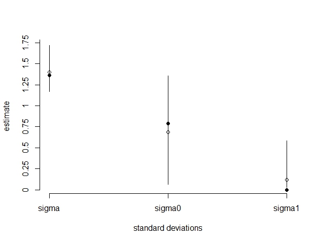
Here is a comparison of the standard deviations between the above model and the nested model from lme4

m2 <- lmer(yN ~ x + (1 |group/indiv), data=qq)
summary(m2)

The summary from this model tells us that

• the standard devation from indiv:group is 0.7909
• the group standard deviation is 0
• the residual deviation is 1.3629

Here is a plot that compares estimates between models. White dots are JAGS estimates, black dots are from lme4, the vertical lines are 95% credible intervals from JAGS.

Additionally, the priors you have set for the precision term of your random effects have most of their mass at zero which will influence the posterior distribution. This is because there are few individuals per group so the data is not outweighing the prior. Note that the credible intervals for sigma0 are the largest out of the three, which reflects uncertainty in this estimate. Setting a dgamma(0.1,0.1) prior returns estimates that are closer to lme4 (if that is your goal).

UPDATE:

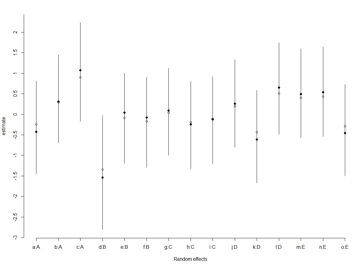
Here is a plot that compares the random effects from the JAGS model to lme4. As with the previous plot. White dots are median estimates from JAGS, black dots are estimates from lme4 via ranef(m2), and vertical lines are 95% credible intervals from JAGS. You can see from this figure that all of the JAGS estimates for the random effects are getting pulled towards zero given that sigma0 is estimated to be smaller.

Here is how I modified the JAGS model to track these random effects as a derived parameter. From there I just added "b_pred" as an additional element to track in the variable.names argument of coda.samples.

st <- "
model {

for(i in 1:n){
mu[i] <- beta[1] + b1[ind[i]] + b2[group[i]] + beta[2]* x[i] 
y[i] ~ dnorm(mu[i], tau)
}

for(i in 1:2){  beta[i] ~ dnorm(0, 0.0001)  }

tau ~ dgamma(0.01, 0.01)
sigma <- sqrt(1/tau) 

# hierarchical model
for (i in 1:nGrp) { b2[i] ~ dnorm(0, tau1) }
for (i in 1:nInd) { b1[i] ~ dnorm(b2[ind_per_group[i]], tau0) }

tau0 ~ dgamma(0.001, 0.001)
sigma0 <- sqrt(1/tau0) 
tau1 ~ dgamma(0.001, 0.001)
sigma1 <- sqrt(1/tau1) 
# calculate random effects
for(i in 1:nInd) {b_pred[i] <- b1[i] + b2[ind_per_group[i]]}

}
"

Onestep

Hi, M_Fidino. Thank you very much for your answer. The way you set the priors was the way I was thinking of the problem: that the indiv are normally distributed around the group they are nested within. However, I don't think this is actually correct. This can be seen by looking at predictions from the lmer model : mod = lmer(yN ~ x + (1 |group/indiv), data=qq) ; ranef(mod) - where there is no sum to zero of these predictions (of indiv within group). The design matrix Z, for the RE's getME(mod, "Z"), I think shows how the data is organised, and I suppose I could pass this, Z, to jags – Snowshed

I think the major difference in the variance / predictions between jags and lme4 is due to a combination of the priors - in jags sigma^2 > 0, but lme4 allows it to equal zero, and the small amount of data. (ps I think using the prior of dgamma(0.1,0.1) is fine if there is prior info that the variance should be small, otherwise I think it would be too precise / informative) – Snowshed

ps I'll let the bounty run for a few more hours iand then award , Thanks again for your help – Snowshed

Hi @user2957945. I'm going to have to disagree with here. These models and nearly identical save for the fact that the Bayesian one cannot allow a variance term to be zero (because of the gamma prior). I'll edit my response to show how the random effects are nearly identical between JAGS and lme4. – Onestep

Hi, yes, I agree they are same. I just think that when the levels are uniquely identified (ie indiv in group) that the model can be specified using the exchangeable priors that i used in my question. – Snowshed