Emtpy factor level with tapply in after_stat causes hodgepodge

Question

I would like to draw a plot with percentage labels per x-axis group. This works fine without empty groups:

# library
library(ggplot2)
library(reshape2)

# example data from reshape2
str(tips)
#> 'data.frame':    244 obs. of  7 variables:
#>  $ total_bill: num  17 10.3 21 23.7 24.6 ...
#>  $ tip       : num  1.01 1.66 3.5 3.31 3.61 4.71 2 3.12 1.96 3.23 ...
#>  $ sex       : Factor w/ 2 levels "Female","Male": 1 2 2 2 1 2 2 2 2 2 ...
#>  $ smoker    : Factor w/ 2 levels "No","Yes": 1 1 1 1 1 1 1 1 1 1 ...
#>  $ day       : Factor w/ 4 levels "Fri","Sat","Sun",..: 3 3 3 3 3 3 3 3 3 3 ...
#>  $ time      : Factor w/ 2 levels "Dinner","Lunch": 1 1 1 1 1 1 1 1 1 1 ...
#>  $ size      : int  2 3 3 2 4 4 2 4 2 2 ...

# function to count percentage per day
comp_pct <- function(count, day) {
  count / tapply(count, day, sum)[day]
}

# correct plot

ggplot(tips, aes(x = day, group = sex)) +
  geom_bar(aes(y = ..prop.., fill = factor(..group..)), stat = "count") +
  geom_text(aes(
    label = after_stat(scales::percent(comp_pct(count, x))),
    y = ..prop..
  ), stat = "count", position = position_stack(vjust = 0.5)) +
  labs(y = "Percent", fill = "sex") +
  scale_x_discrete(drop=FALSE) +
  scale_y_continuous(labels = scales::percent)

However, after adding an empty level, the labelling with after_stat does not work anymore as expected. I am not sure if this is caused by the ordering of the output from the tapply() in comp_pct. However, I am unable to solve it.

# additional empty level
tips -> tips1

tips1$day <- factor(tips$day, levels=c("NewDay",levels(tips$day)))
levels(tips1$day)
#> [1] "NewDay" "Fri"    "Sat"    "Sun"    "Thur"

# bars OK, labels not OK
ggplot(tips1, aes(x = day, group = sex)) +
  geom_bar(aes(y = ..prop.., fill = factor(..group..)), stat = "count") +
  geom_text(aes(
    label = after_stat(scales::percent(comp_pct(count, x))),
    y = ..prop..
  ), stat = "count", position = position_stack(vjust = 0.5)) +
  labs(y = "Percent", fill = "sex") +
  scale_x_discrete(drop=FALSE) +
  scale_y_continuous(labels = scales::percent)
#> Warning: Removed 2 rows containing missing values (geom_text).

^{Created on 2022-04-02 by the reprex package (v2.0.1)}

Lyonnaise

Rather than relying on ggplot's tricky stat functions, why not just pre-calculate what you need and plot that directly? It would also be easier to help if you could provide the output of dput(tips). – Periodate

Thank you. I think it might be quite complex to pre-calculate everything by hand? tips is part of reshape2, a dput would be very long. I added a str. – Lyonnaise

Answer 1

The issue is that using count / tapply(count, day, sum)[day] extracts the computed percentages by position (Sorry. My fault. (;) While this works fine for the original dataset, it does not work in the more general case, i.e. an NA is returned for the fourth bar label:

print(day)
#> [1] 2 3 4 5 2 3 4 5
#>         3         4         5      <NA>         3         4         5      <NA> 
print(count / tapply(count, day, sum)[day])
#> 0.1034483 0.3684211 0.2903226        NA 0.1149425 0.7763158 0.9354839        NA 

To fix that we have to convert day to a character to extract the percentage values by name:

library(ggplot2)
library(reshape2)

# additional empty level
tips -> tips1

# function to count percentage per day
comp_pct <- function(count, day) {
  count / tapply(count, day, sum)[as.character(day)]
}

tips1$day <- factor(tips$day, levels = c("NewDay", levels(tips$day)))

ggplot(tips1, aes(x = day, group = sex)) +
  geom_bar(aes(y = ..prop.., fill = factor(..group..)), stat = "count") +
  geom_text(aes(
    label = after_stat(scales::percent(comp_pct(count, x))),
    y = ..prop..
  ), stat = "count", position = position_stack(vjust = 0.5)) +
  labs(y = "Percent", fill = "sex") +
  scale_x_discrete(drop = FALSE) +
  scale_y_continuous(labels = scales::percent)

Canikin

Answer 2

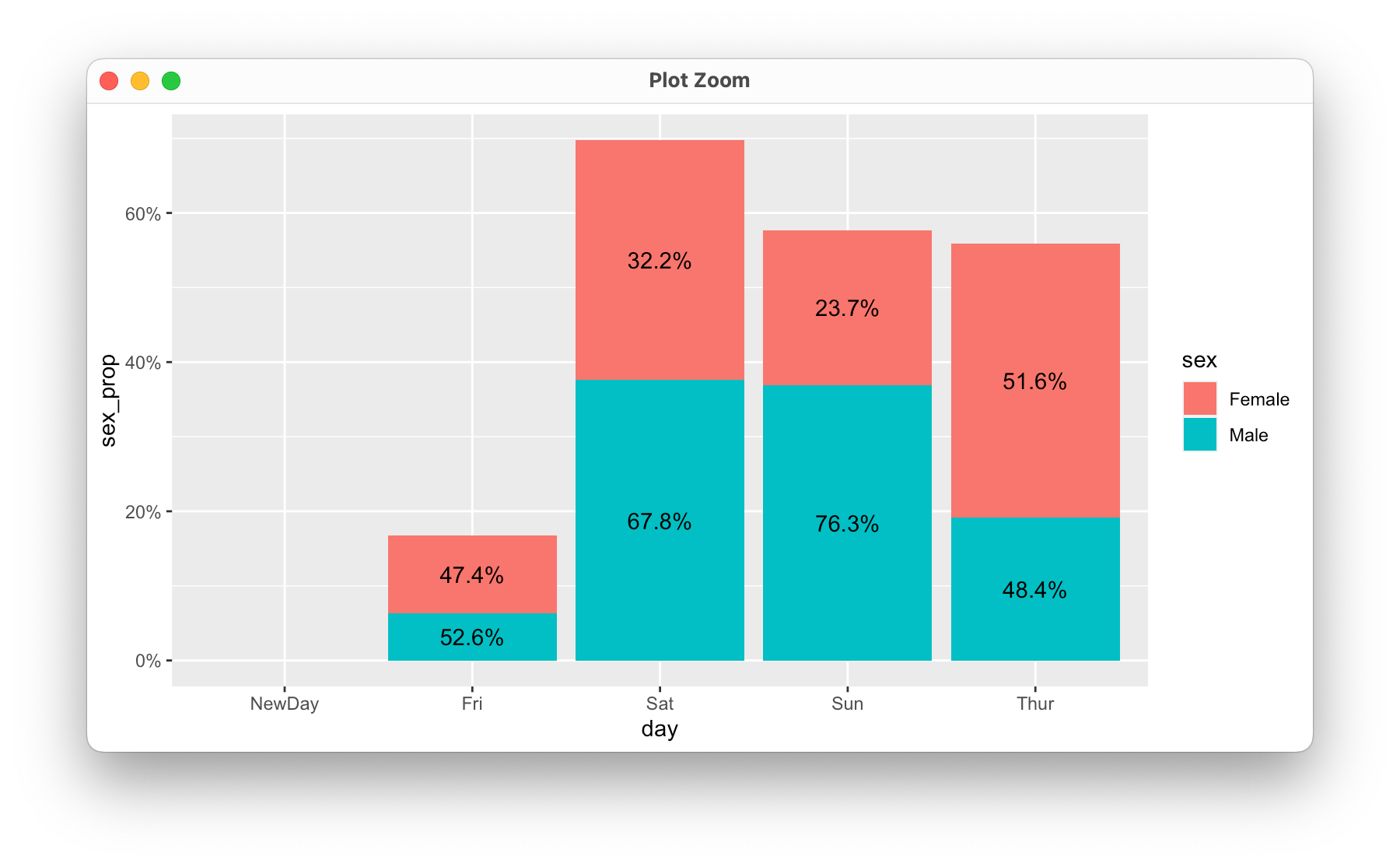
It's much easier to pre-calculate what you'd like to plot rather than trying to wrangle the interactions between ggplot's summary functions. Pre-calculating your statistics also gives you better visibility into your process and more control over the potential outputs (i.e., if you wanted to save the data in a spreadsheet as well). We can calculate the plot contents using the tidyverse packages (of which ggplot is one), which greatly simplifies the plotting:

library(reshape2)
library(tidyverse)

tips1 <- tips

# add new level to day factor
tips1$day <- factor(tips1$day, levels = c('NewDay', levels(tips1$day)))

# calculate what is to be plotted
tips_summary <- tips1 %>% 
  count(day, sex) %>% 
  group_by(day) %>% 
  mutate(prop_day = n / sum(n)) %>% 
  group_by(sex) %>% 
  mutate(prop_sex = n / sum(n))

# plot; scale_x_discrete(drop = F) is necessary to plot the empty NewDay level 
ggplot(tips_summary, aes(x = day, y = prop_sex, fill = sex)) +
  geom_col(position = 'stack') +
  geom_text(aes(label = scales::percent(prop_day)), position = position_stack(vjust = 0.5)) +
  scale_x_discrete(drop = F) +
  scale_y_continuous(labels = scales::percent)

Periodate