Cubic spline implementation in Octave

Question

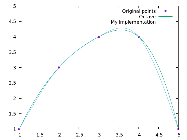
My bold claim is that the Octave implementation of the cubic spline, as implemented in interp1(..., "spline") differs from the "natural cubic spline" algorithm outlined in, e.g., Wolfram's Mathworld. I have written my own implementation of the latter and compared it to the output of the interp1(..., "spline") function, with the following results:

I discovered that when I try the same comparison with 4 points, the solutions also differ, and, moreover, the Octave solution is identical to fitting a single cubic polynomial to all four points (and not actually producing a piecewise spline for the three intervals).

I also tried to look under the hood at Octave's implementation of splines, and found it was too obtuse to read and understand in 5 minutes.

I know that there are a few options for boundary conditions one can choose ("natural" vs "clamped") when implementing a cubic spline. My implementation uses "natural" boundary conditions (in which the second derivative of the two exterior points is set to zero).

If Octave's cubic spline is indeed different to the standard cubic spline, then what actually is it?

EDIT:

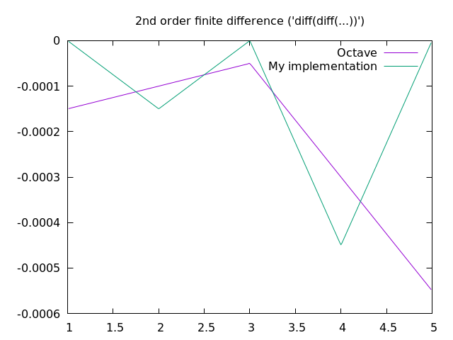
The second order differences of the two solutions shown in the Comparison plot above are plotted here:

Firstly, there appear to be only two cubic polynomials in Octave's case: one that is fit over the first two intervals, and one that is fit over the last two intervals. Secondly, they are clearly not using "natural" splines, since the second derivatives at the extremes do not tend to zero.

Also, I think the fact that the second order difference for my implementation at the middle (i.e. 3rd) point is zero is just a coincidence, and not demanded by the algorithm. Repeating this test for a different set of points will confirm/refute this.

Insomnolence

Without digging into the Octave code myself...Some more possible tests: natural cubic spline between 2 points is a straight line. Between 3 non-col-linear points it should not be a parabola (quadratic). You might be able to compute approximations to the derivatives by using divided differences. Note that the spline should be C2 - that is, the second derivative should be continuous, and piece-wise linear. – Bullivant

I believe the not-a-knot end conditions are used, that is one potential difference: gnu.org/software/octave/doc/v4.0.3/… – Adalbert

That's not natural! The natural spline has - as your implementation shows - 0 second derivative at the ends. The natural spline minimizes (linearized) bending energy over the interval, while interpolating, and it is unique - anything else might minimize a different energy functional, or just be a piece-wise cubic curve. – Bullivant

Answer 1

Different end conditions explains the difference between your implementation and Octave's. Octave uses the not-a-knot condition (depending on input)

See help spline

To explain your observations: the third derivative is continuous at the 2nd and (n-1)th break due to the not-a-knot condition, so that's why Octave's second derivative looks like it has less 'breaks', because it is a continuous straight line over the first two and last two segments. If you look at the third derivative, you can see the effect more clearly - the 3rd derivative is discontinuous only at the 3rd break (the middle)

x = 1:5;
y = rand(1,5);
xx = linspace(1,5);
pp = interp1(x, y, 'spline', 'pp');
yy = ppval(pp, xx);
dyy = ppval(ppder(pp, 3), xx);
plot(xx, yy, xx, dyy);

Also the pp data structure looks like this

pp =

  scalar structure containing the fields:

    form = pp
    breaks =

       1   2   3   4   5

    coefs =

       0.427823  -1.767499   1.994444   0.240388
       0.427823  -0.484030  -0.257085   0.895156
      -0.442232   0.799439   0.058324   0.581864
      -0.442232  -0.527258   0.330506   0.997395

    pieces =  4
    order =  4
    dim =  1
    orient = first

Adalbert