Right method for finding 2-D Spatial Spectrum from CSD

Question

I try to implement the spatial spectrum from the above equation (attached)

Where kX, kY are the grid points in k space, C(w,r) - cross spectral densities between the i'th and j'th sensor(here it is a matrix of size ns * ns >no. of sensors). x, y are distances between the sensors. (nk - grid density for kx, ky)

I look for suitable python implementation of the above equation. I've 34 sensors which generates data of size [row*column]=[n*34]. At first, I've found the cross spectral densities (CSD) of among the data of each sensor. Then 2D DFT is performed of the CSD values to get the spatial spectrum.

*) I'm not sure whether the procedure is correct or not. **) Does the python implementation procedure correct? ***) Also, if someone provides some relevant tutorial/link, it will also be helpful for me.

import numpy as np
from scipy import signal
import matplotlib.pyplot as plt
import cmath

# Finding cross spectral density (CSD)
fs=500
def csdMat(data):
    rows, cols = data.shape
    total_csd = []
  
    for i in range(cols):
 
        for j in range(cols):
            f, Pxy = signal.csd(data[:,i], data[:,j], fs, nperseg=512)
            abs_csd = np.abs(Pxy)
            total_csd.append(abs_csd)                     # output as list
            csd_mat = np.array(total_csd)
    return csd_mat

## Spatial Spectra:- DFT of the csd along two dimension

def DFT2D(data):
    #data = np.asarray(data)
    dft2d = np.zeros((M,N), dtype=complex)
    for k in range(len(kx)):
        for l in range(len(ky)):
            sum_matrix = 0.0
            for m in range(M):
                for n in range(N):
                    e = cmath.exp(- 1j * ((kx[k] * dx[m]) / len(dx) + (ky[l] * dy[n]) / len(dy)))
                    sum_matrix +=  data[m,n] * e
            dft2d[k,l] = sum_matrix
    return dft2d

raw_data=np.reshape(np.random.rand(10000*34),(10000,34))

# Call the seismic array
#** Open .NPY files as an array 
#with open('res_array_1000f_131310.npy', 'rb') as f:
#    arr= np.load(f)
#raw_data = arr[0:10000, :]

#CSD of the seismic data
csd = csdMat(raw_data)
print('Shape of CSD data', csd.shape)

# CSD data of a specific frequency
csd_dat=csd[:, 11]  
fcsd = np.reshape(csd_dat, (-1, 34))
fcsd.shape

n = 34
f = 10  # frequency in Hz
c = 50  # wave speed 50, 80, 100, 200  m/s
k = 2.0*np.pi*f/c  # wavenumber
nx = n  # grid density
ny = n
kx = np.linspace(-k,k,nx)  # space vector
ky=  np.linspace(-k,k,ny)   # space vector

# Distance[Meter] between sensors 
x = [2.1,2.1,-0.7,-2.1,-2.1,-0.7,-0.7,0.6,-5.7,-8.5,-11.4,-7.7,-6.3,-3.5,-2.1,-3.4,5.4,-5.2,-8.9,-10,-10,5.4,5.4,-0.8,-3.6,-6.2,-6.8,-12.2,-17.1,-19,-18.6,-13.5,14.8,14.8]
y = [6.65,4.15,3.65,5.05,7.25,8.95,11.85,8.95,-2,-0.6,-0.9,1.25,2.9,0.9,-0.1,-1.4,9.2,5.2,4.8,6.1,8.9,13.3,17.1,17.9,13.8,-9.3,-5.2,-3.6,-3.6,-0.9,3.7,3.7,-1.8,5.7]

dx = np.array(x);  M = len(dx)
dy = np.array(y) ; N = len(dy)
X,Y = np.meshgrid(kx, ky)

dft = DFT2D(fcsd)  # Data or cross-correlation matrix
spec = dft.real    # Spectrum or 2D_DFT of data[real part]

spec = spec/spec.max()

plt.figure()
c = plt.imshow(spec, cmap ='seismic', vmin = spec.min(), vmax = spec.max(),
                 extent =[kx.min(), kx.max(), ky.min(), ky.max()],
                interpolation ='nearest', origin ='lower')
plt.colorbar(c)
plt.rcParams.update({'font.size': 18})
plt.xlabel("Wavenumber, $K_x$ [rad/m]", fontsize=18)
plt.ylabel("Wavenumber,$K_y$ [rad/m]", fontsize=18)
plt.title(f'Spatial Spectrum @10Hz', weight="bold")


#c = Wave Speed; 50, 80,100,200
cc = 2*np.pi*f /c *np.cos(np.linspace(0, 2*np.pi, 34)) 
cs = 2*np.pi*f /c *np.sin(np.linspace(0, 2*np.pi, 34))
plt.plot(cc,cs)

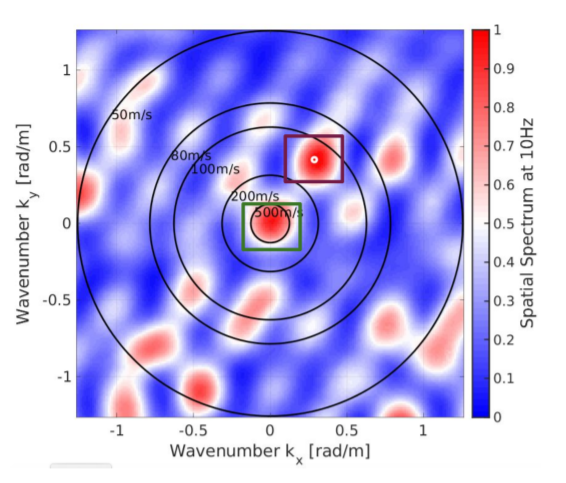
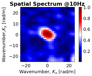
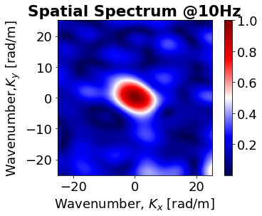
I want to generate the figure as Fig. 01 below However, by using improved code I get the figure with higher resolution as Fig. 02 which is different from Fig. 01.

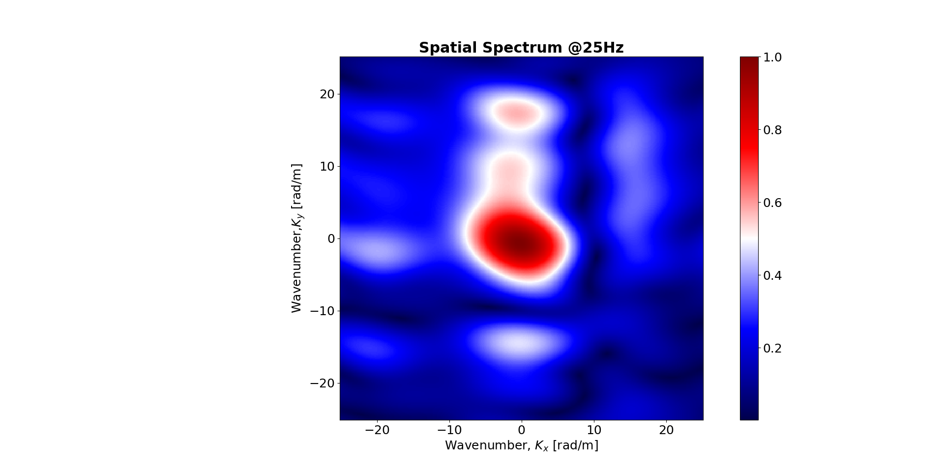
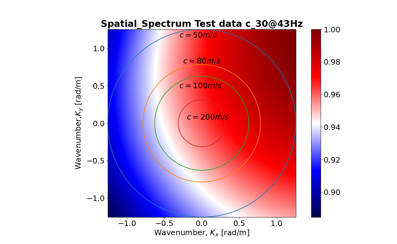
I've added another two figures to compare with the Fig. 01. When consider the range [-k, k], the plot looks like Fig. 03 which is analogous [w.r.t. XY-axis] to Fig. 01, I think this figure is OK except some K-space missed. I hope here exist an issue that need to be fixed.

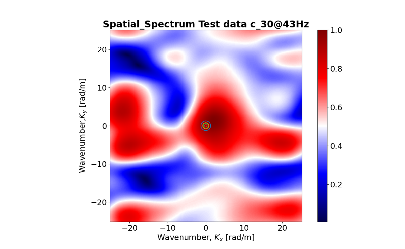
In Fig. 04, we consider the k-space range [-20k, 20k], which looks good but don't have similar axis as of Fig. 01.

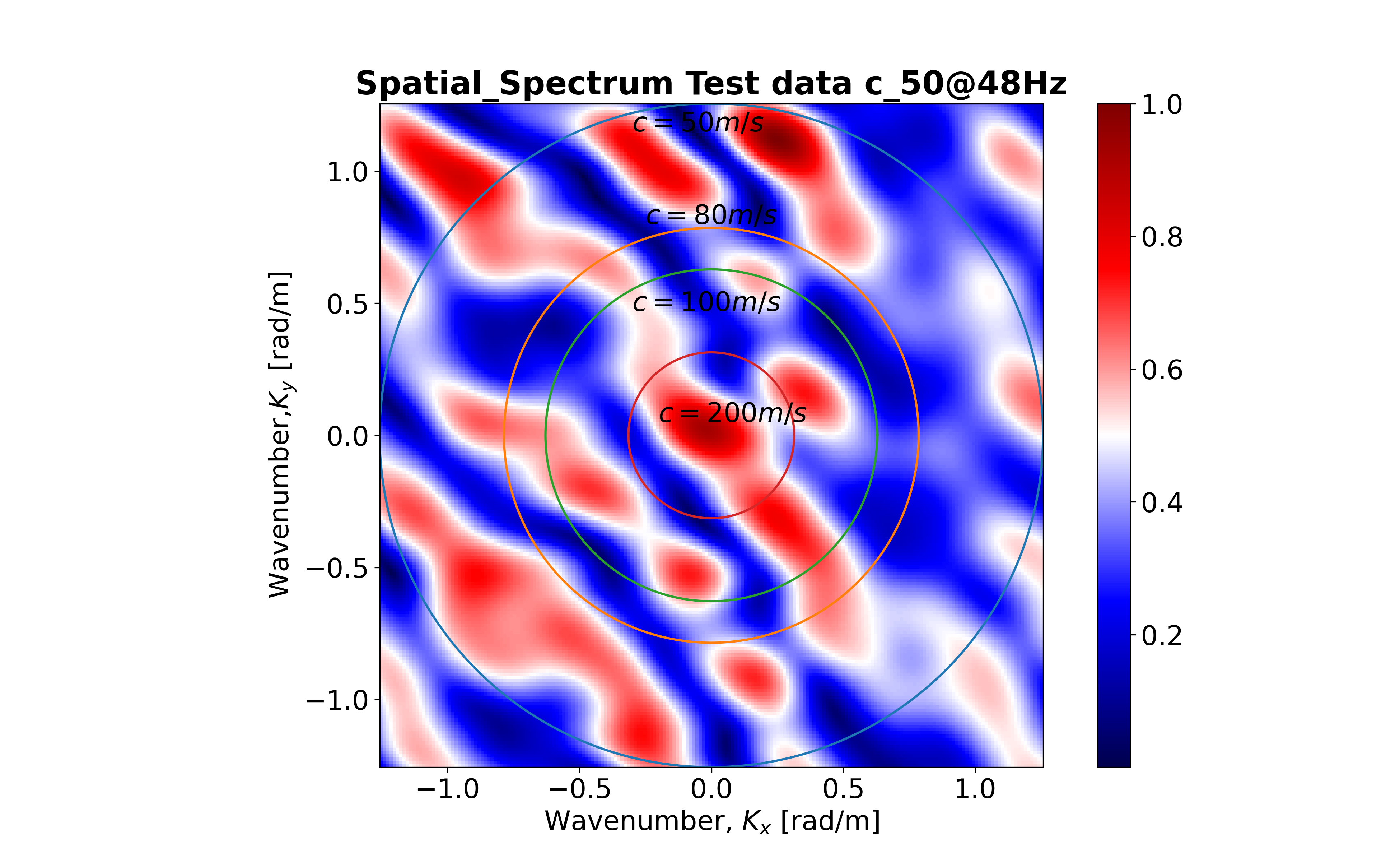
I've put the update Figure as follows: Can anyone help me to generate the figure 01 or similar type? I'm confused about the Figure 02. Can anybody help to make me understand? Thanks in advance.

Janik

Why do you do spec = dft.real # Spectrum or 2D_DFT of data[real part] ? The spectrum is more like np.abs(dft) than just the real part of the DFT. – Une

@PeterK. Thanks. I've changed the DFT value from real to absolute. However, with the above script, I got the plot as of Fig. 02, but I want to generate Fig. 01. Also, Can you suggest how to increase the resolution of the plot? – Janik

Also, in the colorbar, the initial value doesn't start from 0. What is the reason? – Janik

OK. Looking at it again... why do you also take the real part here: real_csd = np.real(Pxy) The cross-spectral density will be complex. Just taking the real part drops information. However, that doesn't fix the problem. – Une

Thanks, now I consider the absolute value of CSD than real part of it. – Janik

@PeterK. What is the data size you have chosen to generate the plot. Your plot looks different from mine. – Janik

Added the full code I used to generate the plot. It's in the repo here – Une

Can you help me to enhance the image resolution? I'm confused how to increase the resolution. Also, is it possible to get the same results by using built-in function for 2d DFT ? – Janik

@PeterK. How to find the amplitude of spectrum, spec = np.abs(dft) ? I f I consider spec/(sampling frequency (fs)*len(kx)*len(ky)*M*N) is that correct? – Janik

I'm not sure! yes, you'll need to use np.abs to get the absolute value. DFTs are generally defined in pairs (forward and inverse). Some people put the scaling on the forward, but most put it on the inverse. Some put the scaling (square-rooted) on both. – Une

@PeterK. As I need to calculate the amplitude in the above spatial spectrum, so I use 2 steps:-i) CSD-> here the scaling would be done by dividing the length of the signal and ii) DFT-> here scaling can be done by dividing the size of the matrix. So, I use spec/(Signal length(L) *len(kx)*len(ky)*M*N). Also, what will be the unit of the amplitude? Again, how to find the unit of amplitude is (ms)^2/Hertz? – Janik

Answer 1

It looks to me like you're zooming in on the central lobe. This would also explain why the scale doesn't go from 0 to 1.

If I change these lines:

kx = np.linspace(-20*k,20*k,nx)  # space vector
ky=  np.linspace(-20*k,20*k,ny)   # space vector

then I get

which looks closer to what you're looking for.

To improve the resolution, I've done a bit of rewriting to get this new picture. See updated code below.

NOTE: I am still not certain this is doing the right thing.

---

Code I used

# Code from https://mcmap.net/q/1772844/-right-method-for-finding-2-d-spatial-spectrum-from-csd

import numpy as np
from scipy import signal
import matplotlib.pyplot as plt
import cmath

# Set up data
# Distance[Meter] between sensors 
x = [2.1,2.1,-0.7,-2.1,-2.1,-0.7,-0.7,0.6,-5.7,-8.5,-11.4,-7.7,-6.3,-3.5,-2.1,-3.4,5.4,-5.2,-8.9,-10,-10,5.4,5.4,-0.8,-3.6,-6.2,-6.8,-12.2,-17.1,-19,-18.6,-13.5,14.8,14.8]
y = [6.65,4.15,3.65,5.05,7.25,8.95,11.85,8.95,-2,-0.6,-0.9,1.25,2.9,0.9,-0.1,-1.4,9.2,5.2,4.8,6.1,8.9,13.3,17.1,17.9,13.8,-9.3,-5.2,-3.6,-3.6,-0.9,3.7,3.7,-1.8,5.7]

if (len(x) != len(y)):
    raise Exception('X and Y lengthd differ')

n = len(x)
dx = np.array(x);  M = len(dx)
dy = np.array(y) ; N = len(dy)

np.random.seed(12345)
raw_data=np.reshape(np.random.rand(10000*n),(10000,n))

f = 10  # frequency in Hz
c = 50  # wave speed 50, 80, 100, 200  m/s
k = 2.0*np.pi*f/c  # wavenumber
kx = np.linspace(-20*k,20*k,n*10)  # space vector
ky=  np.linspace(-20*k,20*k,n*10)   # space vector


# Finding cross spectral density (CSD)
fs=500
def csdMat(data):
    rows, cols = data.shape
    total_csd = []
  
    for i in range(cols):
        for j in range(cols):
            f, Pxy = signal.csd(data[:,i], data[:,j], fs, nperseg=512)
            #real_csd = np.real(Pxy)
            total_csd.append(Pxy)                     # output as list
            
    return np.array(total_csd)

## Spatial Spectra:- DFT of the csd along two dimension

def DFT2D(data):
    #data = np.asarray(data)
    dft2d = np.zeros((len(kx),len(ky)), dtype=complex)
    for k in range(len(kx)):
        for l in range(len(ky)):
            sum_matrix = 0.0
            for m in range(M):
                for n in range(N):
                    e = cmath.exp(- 1j * ((kx[k] * dx[m]) / len(dx) + (ky[l] * dy[n]) / len(dy)))
                    sum_matrix +=  data[m,n] * e
            dft2d[k,l] = sum_matrix
    return dft2d


# Call the seismic array
#** Open .NPY files as an array 
#with open('res_array_1000f_131310.npy', 'rb') as f:
#    arr= np.load(f)
#raw_data = arr[0:10000, :]

#CSD of the seismic data
csd = csdMat(raw_data)
print('Shape of CSD data', csd.shape)

# CSD data of a specific frequency
csd_dat=csd[:, 11]  
fcsd = np.reshape(csd_dat, (-1, n))

dft = DFT2D(fcsd)  # Data or cross-correlation matrix
spec = np.abs(dft) #dft.real    # Spectrum or 2D_DFT of data[real part]

spec = spec/spec.max()

plt.figure()
c = plt.imshow(spec, cmap ='seismic', vmin = spec.min(), vmax = spec.max(),
                 extent =[kx.min(), kx.max(), ky.min(), ky.max()],
                interpolation ='nearest', origin ='lower')
plt.colorbar(c)
plt.rcParams.update({'font.size': 18})
plt.xlabel("Wavenumber, $K_x$ [rad/m]", fontsize=18)
plt.ylabel("Wavenumber,$K_y$ [rad/m]", fontsize=18)
plt.title(f'Spatial Spectrum @10Hz', weight="bold")

Une

Thanks again. Here you consider the enlarged 2-D space [-20, 20] . In the Fig. 01, probably they do some normalization. But, I've no idea how to do the normalization in space? Also, in Fig. 01, it is seen that the 'red blobs' are in motion (it depends on data, though). – Janik

As I've 34 sensors, so I get the CSD matrix of size 34*34, so the resolution is not good enough. Could you please suggest me how to increase the resolution of the plot so that the figure looks smooth? – Janik

@Janik See update with a slight re-write of your code to get improved resolution. – Une

Oh, great. Just increase the grid density results in the higher resolution. It helps me more. – Janik

@Janik The original code tied the point density in k-space to the number of sensors. The two don’t need to be connected. The updated code removes the connection and allows for arbitrary (if computationally expensive) resolution. – Une

Also, I'm interested in Fig. 01 where they consider all the space [seismic array mounted] within the boundary [-1, 1] while in my case the boundary is [-20, 20]. I've confusion at this point. As this approach is computationally expensive, is there any option to make the procedure faster? I mean, is it possible to use any built-in function in python? Thanks – Janik

Also, I'm interested in Fig. 01 where they consider all the space of interest [where seismic sensor array mounted] within the boundary [-1, 1] while in my case the boundary is [-20, 20]. I've confusion at this point. Another query from my side, as this approach is computationally expensive, is there any option to make the procedure faster? I mean, is it possible to use any built-in function in python? Thanks – Janik

Another point, to find the wavenumber space vector [kx, ky], I consider frequency, f=10 hz; k=2*pi*f/c while during CSD calculation I got csd values correspond to various frequencies f, Pxy = signal.csd(dset_X, dset_Y, fs=fs, window='hann', nperseg=nperseg, noverlap=None, nfft=nfft) which gives me the range of 1Hz to 250 Hz. So, first I assume 'f=10 hz' and later I get range of frequencies from CSD, so which frequency I'll consider finally. Can you please explain this point? Thanks – Janik

No time today. Will try again tomorrow, but it’ll probably be Wednesday before I get back to this. – Une

wavenumber k=2*pi/lambda=2*pi*f/c f= frequency & c= speed of the wave vector; In Fig.01, they consider [-k, k] for space of interest while we consider [-20k, 20k] the space of interest. I've doubt that something is missing unconsciously. – Janik

Ok, I replaced the value of e in the above code with e = cmath.exp(-1j*(float(kx[k]* dx[m]) + float(ky[l]*dy[n]))) which aligns with the above equation and the axis problem is solved, shown in Fig. 05. – Janik

Could you please help me to interpret the Fig. 03. From the fig. 03, so far I understand the wave vector is moving from the center. Is that right? Also, is it possible to conclude from the fig. 03 that how many dominant mode of propagation has seen from the figure? Thanks. – Janik

Answer 2

As per above equation, the script for the spatial spectrum is better match as follows. The function of the "DFT2D()" is modified here which satisfy the equation.

    def DFT2D(data):

        P=len(kx)
        Q=len(ky)
        dft2d = np.zeros((P,Q), dtype=complex)
        for k in range(P):
            for l in range(Q):
                sum_matrix = 0.0
                for m in range(M):
                    for n in range(N): #
                        e = cmath.exp(-1j*(float(kx[k]*(dx[m]-dx[n])+ float(ky[l]*(dy[m]-dy[n])))))#* cmath.exp(-1j*w*t[n]))
                        sum_matrix += data[m, n] * e
                        #print('sum matrix would be', sum_matrix)
                #print('sum matrix would be', sum_matrix)
                dft2d[k,l] = sum_matrix
         return dft2d

Litharge