Exponential decay curve fitting in numpy and scipy

Question

I'm having a bit of trouble with fitting a curve to some data, but can't work out where I am going wrong.

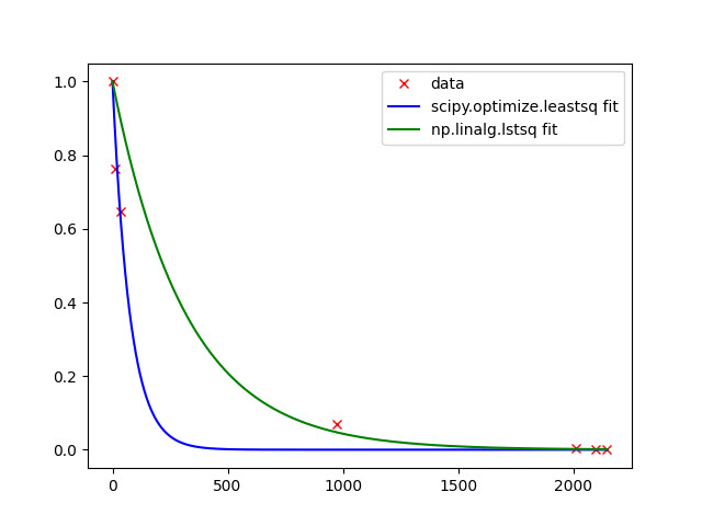
In the past I have done this with numpy.linalg.lstsq for exponential functions and scipy.optimize.curve_fit for sigmoid functions. This time I wished to create a script that would let me specify various functions, determine parameters and test their fit against the data. While doing this I noticed that Scipy leastsq and Numpy lstsq seem to provide different answers for the same set of data and the same function. The function is simply y = e^(l*x) and is constrained such that y=1 at x=0.

Excel trend line agrees with the Numpy lstsq result, but as Scipy leastsq is able to take any function, it would be good to work out what the problem is.

import scipy.optimize as optimize
import numpy as np
import matplotlib.pyplot as plt

## Sampled data
x = np.array([0, 14, 37, 975, 2013, 2095, 2147])
y = np.array([1.0, 0.764317544, 0.647136491, 0.070803763, 0.003630962,     0.001485394,     0.000495131])

# function
fp = lambda p, x: np.exp(p*x)

# error function
e = lambda p, x, y: (fp(p, x) - y)

# using scipy least squares
l1, s =  optimize.leastsq(e, -0.004, args=(x,y))
print l1
# [-0.0132281]


# using numpy least squares
l2 = np.linalg.lstsq(np.vstack([x, np.zeros(len(x))]).T,np.log(y))[0][0]
print l2
# -0.00313461628963 (same answer as Excel trend line)

# smooth x for plotting
x_ = np.arange(0, x[-1], 0.2)

plt.figure()
# plt.plot(x, y, 'rx', x_, fp(l1, x_), 'b-', x_, fp(l2, x_), 'g-')
plt.plot(x, y, 'rx', label= 'data')
plt.plot(x_, fp(l1, x_), 'b-', label= 'scipy.optimize.leastsq fit')
plt.plot(x_, fp(l2, x_), 'g-', label= 'np.linalg.lstsq fit')
plt.legend()
plt.show()

Edit - additional information

The MWE above includes a small sample of the dataset. When fitting the actual data the scipy.optimize.curve_fit curve presents an R^2 of 0.82, while the numpy.linalg.lstsq curve, which is the same as that calculated by Excel, has an R^2 of 0.41.

Dismiss

perhaps some linearization is needed or here – Morley

Answer 1

You are minimizing different error functions.

When you use numpy.linalg.lstsq, the error function being minimized is

np.sum((np.log(y) - p * x)**2)

while scipy.optimize.leastsq minimizes the function

np.sum((y - np.exp(p * x))**2)

The first case requires a linear dependency between the dependent and independent variables, but the solution is known analitically, while the second can handle any dependency, but relies on an iterative method.

On a separate note, I cannot test it right now, but when using numpy.linalg.lstsq, I you don't need to vstack a row of zeros, the following works as well:

l2 = np.linalg.lstsq(x[:, None], np.log(y))[0][0]

Pimp

Thanks @Pimp - great answer! Unfortunately my maths knowledge is not that great; is one write or wrong [also see edit above], or are they just fundamentally different...? What are the implications for other functions, for example, if I wanted test the fit of a Sigmoid or Gompertz curve to the same data? – Dismiss

@Dismiss I don't have the knowledge to properly answer your question, but I am pretty sure that fitting an exponential as you did with np.linalg.lstsq is just a quick'n'dirty trick that doesn't compute errors properly. There's some discussion (hard for me to follow) here: mathworld.wolfram.com/LeastSquaresFittingExponential.html If you don't want to dive really deep into this stuff, I'd go with scipy's method for everything: it should give better fits, and your results will be consistent for all functions. – Pimp

thanks again! I have done some more research on this and, as you mentioned, have found that the np.linalg.lstsq method overly weights y-errors at low x values. The link you shared, and some other resources I found, allowed me to derive one other analytical method (the thing that makes it tricky is the constraint --- all the books describe the method for y=ae^bx rather than y=e^b*x), however, this also produces a worse fitting curve than the iterative scipy.optimize.leastsq. – Dismiss

@ Jaime: np.ones works for intercept x2= np.vstack([x, np.ones(len(x))]).T; l2 = np.linalg.lstsq(x2, np.log(y), rcond=-1)[0]; print( "slope, intercept: ", l2) and come back from linearized form to the exponential y_2 = np.exp(l2[1]) * np.exp(l2[0] * x_) to use it in normal non-lorarithmic y-axis scale of plot plt.plot( x_, y_2, 'g-', label= "np.linalg.lstsq fit"); plt.legend(); -- you'll get identical plot that OP have got – Morley

Answer 2

To expound a bit on Jaime's point, any non-linear transformation of the data will lead to a different error function and hence to different solutions. These will lead to different confidence intervals for the fitting parameters. So you have three possible criteria to use to make a decision: which error you want to minimize, which parameters you want more confidence in, and finally, if you are using the fitting to predict some value, which method yields less error in the interesting predicted value. Playing around a bit analytically and in Excel suggests that different kinds of noise in the data (e.g. if the noise function scales the amplitude, affects the time-constant or is additive) leads to different choices of solution.

I'll also add that while this trick "works" for exponential decay to 0, it can't be used in the more general (and common) case of damped exponentials (rising or falling) to values that cannot be assumed to be 0.

Catbird

Answer 3

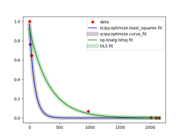
of course, possibility to linearize data (your case) and use of LS-approach log_transformed_fit here is always faster and for full-rank and well-conditioned(not singular) matrices gives best fit (as it is BLUE). Linear Algebra is always comparably fast in numpy and scipy. Non-linear approximation using finite-differences is the last choice from speed viewpoint. If you can provide explicitly jac and hess functions for non-linear approximation, of course you will benefit for speed. Using non-linear approximation with many of scipy.optimize methods you always have threat to stack in local minimum under certain chosen init_guess_params -- therefore only convex functions with one optimum value can give correct resulted parameters. Otherwise, you can just choose more suitable method from those available in scipy.optimize-package. For global min/max in scipy.optimize-package other functions exist. So everything, as usually, depends on Data, Task and Solver. For the use of scipy.optimize.least_squares can try to vary loss and f_scale depending on data. Of course, statistical scores (e.g. goodness-of-fit etc) can help to choose the best solver (for best fit). But again, OLS gives BLUE estimates and for the predictive ability model should be efficient and consistent as well, you have small size of sample. For your data linear and non-linear fitting looks like this:

import scipy.optimize as optimize
import numpy as np
import matplotlib.pyplot as plt

## Sampled data
x = np.array([0, 14, 37, 975, 2013, 2095, 2147])
y = np.array([1.0, 0.764317544, 0.647136491, 0.070803763, 0.003630962,     0.001485394,     0.000495131])

x_ = np.arange(x.min(), x.max(), 0.2)   # grid for plot

plt.figure()
plt.plot(x, y, 'ro', label= 'data')

################################### Normal Equation

##a = np.vstack([x, np.ones(len(x))]).T
##print(np.dot(np.linalg.inv(np.dot(a.T, a)), np.dot(a.T, y)))

###################################
## scipy.optimize FOR NON-LINEAR APPROX.
################################### scipy.optimize.least_squares
# function
fp = lambda a, p, x: a * np.exp(p*x)

# error function
e = lambda p, x, y: (y - fp(*p, x) )

# using scipy least squares
res =  optimize.least_squares(e, [0., 0.], args=(x,y), )
##print( res)
l1 = res.x
print( l1)

plt.plot(x_, fp(*l1, x_), 'b-', label= 'scipy.optimize.least_squares fit')

##full_output
##popt, pcov, info, mesg, ler  = optimize.leastsq(residual, p0, args=(x, y), full_output=True)
##print("popt, pcov, info, mesg, ler: ", popt, pcov, info, mesg, ler)

####################################### scipy.optimize.curve_fit
##if p0=(1, 1) then
##RuntimeWarning: overflow encountered in exp:  return a*np.exp(-c*x)

from scipy.optimize import curve_fit
def func(x, a, c):
    return a*np.exp(c*x)

popt, pcov = curve_fit(func, x, y, p0=(1, 0))
print(popt)
y_cf = func(x_, *popt)
plt.plot(x_, y_cf, 'k-', linewidth= 10, label= 'scipy.optimize.curve_fit', alpha=0.2 )

####################################
## LS FOR LINEAR PARAMS
#################################### np.linalg.lstsq
# using numpy least squares
xr, residuals, rank, s = np.linalg.lstsq(np.vstack([x, np.ones(len(x))]).T, np.log(y), rcond=-1)
##print("x, residuals, rank, s: ", x, residuals, rank, s)
l2= xr
print( "slope, intercept: ",  l2)
# ..........  (same answer as Excel trend line)

y_2 = np.exp(l2[1]) * np.exp(l2[0] * x_)
plt.plot(x_, y_2, 'g-', label= 'np.linalg.lstsq fit')

#################################### statsmodels
import statsmodels.api as sm

X = sm.add_constant(x)
model = sm.OLS(np.log(y), X)
result = model.fit()

intercept_OLS, slope_OLS = result.params
print('OLS: ', slope_OLS, intercept_OLS,)

y_3 = np.exp(intercept_OLS)  * np.exp( slope_OLS * x_)
plt.plot(x_, y_3, 'g-', label= 'OLS fit', linewidth= 10,  alpha=0.2)

plt.legend()
plt.show() 

with data from the example from docs plot will be significantly different

Normalizing data and then Linearizing y=Ae^(Bx) taking logarithm from both sides lny=lnA+Bx gives the possibility to use least-squares from scipy.optimize

xxx= x
yyy= np.log(y)

# model function
model = lambda a, b, x: (np.log(a) + b*x)

# error function
def e ( p, x, y):  return (y - model(*p, x) )    #**2

# using scipy least squares
params =  optimize.least_squares(e, [1., 0.], args=(xxx,yyy), ).x

plt.plot(x_, np.exp(model(*params, x_)), 'm-', label= ' scipy.optimize.least_squares for linearized data'); plt.legend()

p.s. other linearization techniques

Morley