Finding straight lines from tightly coupled lines and noise curvy lines

Question

I have this image for a treeline crop. I need to find the general direction in which the crop is aligned. I'm trying to get the Hough lines of the image, and then find the mode of distribution of angles.

I've been following this tutorialon crop lines, however in that one, the crop lines are sparse. Here they are densely pack, and after grayscaling, blurring, and using canny edge detection, this is what i get

import cv2
import numpy as np
import matplotlib.pyplot as plt

img = cv2.imread('drive/MyDrive/tree/sample.jpg')
gray = cv2.cvtColor(img, cv2.COLOR_RGB2GRAY)
gauss = cv2.GaussianBlur(gray, (3,3), 3)

plt.figure(figsize=(15,15))
plt.subplot(1,2,1)
plt.imshow(gauss)

gscale = cv2.Canny(gauss, 80, 140)
plt.subplot(1,2,2)
plt.imshow(gscale)
plt.show()

(Left side blurred image without canny, left one preprocessed with canny)

After that, I followed the tutorial and "skeletonized" the preprocessed image

size = np.size(gscale)

skel = np.zeros(gscale.shape, np.uint8)

ret, gscale = cv2.threshold(gscale, 128, 255,0)
element = cv2.getStructuringElement(cv2.MORPH_CROSS, (3,3))
done = False

while not done:
  eroded = cv2.erode(gscale, element)
  temp = cv2.dilate(eroded, element)
  temp = cv2.subtract(gscale, temp)
  skel = cv2.bitwise_or(skel, temp)
  gscale = eroded.copy()
  
  zeros = size - cv2.countNonZero(gscale)
  if zeros==size:
    done = True

Giving me

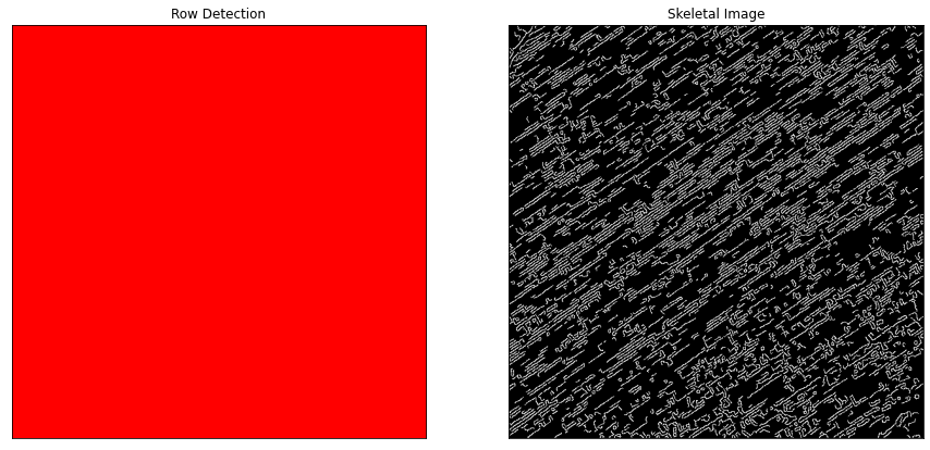
As you can see, there are a bunch of curvy lines still. When using the HoughLines algorithm on it, there are 11k lines scattered everywhere

lines = cv2.HoughLinesP(skel,1,np.pi/180,130)
a,b,c = lines.shape
for i in range(a):
    rho = lines[i][0][0]
    theta = lines[i][0][1]    
    a = np.cos(theta)
    b = np.sin(theta)
    x0 = a*rho
    y0 = b*rho
    x1 = int(x0 + 1000*(-b))
    y1 = int(y0 + 1000*(a))
    x2 = int(x0 - 1000*(-b))
    y2 = int(y0 - 1000*(a))
    cv2.line(img,(x1,y1),(x2,y2),(0,0,255),2, cv2.LINE_AA)#showing the results:

plt.figure(figsize=(15,15))
plt.subplot(121)#OpenCV reads images as BGR, this corrects so it is displayed as RGB
plt.plot()
plt.imshow(cv2.cvtColor(img, cv2.COLOR_BGR2RGB)) 
plt.title('Row Detection')
plt.xticks([])
plt.yticks([])
plt.subplot(122)
plt.plot()
plt.imshow(skel,cmap='gray')
plt.title('Skeletal Image')
plt.xticks([])
plt.yticks([])
plt.show()

I am a newbie when it comes to cv2, so I have 0 clue what to do. Searched and tried a bunch of stuff but none works. How can I remove the mildly big dots, and remove the squiggly lines?

Lozengy

hey, this can be phrased as more of an image processing problem than a programming problem. If you don't find an answer here, maybe migrate the question over to signals.stackexchange.com :) – Sekofski

Looks like Fourrier transform might be useful here. – Sheffield

You could try median of Sobel angle – Eventuality

@Sheffield I know what fourier transform is, but I dont know how it could help, could you explain? – Lozengy

@Eventuality I'll figure how to do that out – Lozengy

@MarcusMüller Thanks, i'll try it out :^) – Lozengy

Answer 1

You can use a 2D FFT to find the general direction in which the crop is aligned (as proposed by mozway in the comments). The idea is that the general direction can be easily extracted from centred beaming rays appearing in the magnitude spectrum when the input contains many lines in the same direction. You can find more information about how it works in this previous post. It works directly with the input image, but it is better to apply the Gaussian + Canny filters.

Here is the interesting part of the magnitude spectrum of the filtered gray image:

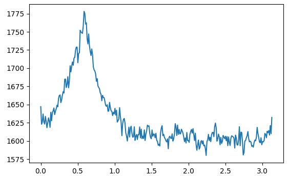
The main beaming ray can be easily seen. You can extract its angle by iterating over many lines with an increasing angle and sum the magnitude values on each line as in the following figure:

Here is the magnitude sum of each line plotted against the angle (in radian) of the line:

Based on that, you just need to find the angle that maximize the computed sum.

Here is the resulting code:

def computeAngle(arr):
    # Naive inefficient algorithm
    n, m = arr.shape
    yCenter, xCenter = (n-1, m//2-1)
    lineLen = m//2-2
    sMax = 0.0
    bestAngle = np.nan
    for angle in np.arange(0, math.pi, math.pi/300):
        i = np.arange(lineLen)
        y, x = (np.sin(angle) * i + 0.5).astype(np.int_), (np.cos(angle) * i + 0.5).astype(np.int_)
        s = np.sum(arr[yCenter-y, xCenter+x])
        if s > sMax:
            bestAngle = angle
            sMax = s
    return bestAngle

# Load the image in gray
img = cv2.imread('lines.jpg')
gray = cv2.cvtColor(img, cv2.COLOR_RGB2GRAY)

# Apply some filters
gauss = cv2.GaussianBlur(gray, (3,3), 3)
gscale = cv2.Canny(gauss, 80, 140)

# Compute the 2D FFT of real values
freqs = np.fft.rfft2(gscale)

# Shift the frequencies (centering) and select the low frequencies
upperPart = freqs[:freqs.shape[0]//4,:freqs.shape[1]//2]
lowerPart = freqs[-freqs.shape[0]//4:,:freqs.shape[1]//2]
filteredFreqs = np.vstack((lowerPart, upperPart))

# Compute the magnitude spectrum
magnitude = np.log(np.abs(filteredFreqs))

# Correct the angle
magnitude = np.rot90(magnitude).copy()

# Find the major angle
bestAngle = computeAngle(magnitude)

Sharice

Very nice, cheers ;) – Sheffield

Excuse the language, but HOLY SHIT IT ACTUALLY WORKED, I WAS HONESTLY NOT EXPECTING MUCH, THIS IS ACTUALLY AMAZING, THANK YOU SO MUCH SIR – Lozengy

And thanks a lot for the well written answer, one of the bests i've ever seen – Lozengy

Answer 2

Just for completeness I would like to post the Sobel Gradient Angle way as well.

General idea:

1. for every pixel, compute X and Y gradient (e.g. with Sobel)
2. Compute the angle from the X and Y gradient information and their distribution
3. find the modes e.g. with a histogram and select the highest one

Written in C++ but probably easily convertable to python:

int main()
{
    try
    {
        cv::Mat img = cv::imread("C:/data/StackOverflow/cropLines/lines.jpg", cv::IMREAD_GRAYSCALE);

        // tests with artificial lines:
        //img = cv::Mat::zeros(img.size(), CV_8UC1);
        //img = cv::Mat(img.size(), CV_8UC1, cv::Scalar::all(255));
        //cv::line(img, cv::Point(0, img.rows), cv::Point(img.cols, 0), cv::Scalar::all(255), 10); // sample to check angles
        //cv::line(img, cv::Point(img.cols, img.rows), cv::Point(0, 0), cv::Scalar::all(255), 10); // sample to check angles
        //cv::line(img, cv::Point(img.cols, img.rows/2), cv::Point(0, img.rows/2), cv::Scalar::all(255), 10); // sample to check angles
        //cv::line(img, cv::Point(img.cols/2, img.rows), cv::Point(img.cols/2, 0), cv::Scalar::all(255), 10); // sample to check angles
        //cv::line(img, cv::Point(img.cols / 2, img.rows), cv::Point(img.cols / 2, 0), cv::Scalar::all(255), 10); // sample to check angles
        //cv::line(img, cv::Point(img.cols / 2, img.rows), cv::Point(img.cols / 2, 0), cv::Scalar::all(0), 10); // sample to check angles
        cv::imshow("img", img);

        cv::Mat gradX, gradY, mag, angle;
        cv::Sobel(img, gradX, CV_32F, 1, 0, 3);
        cv::Sobel(img, gradY, CV_32F, 0, 1, 3);

        cv::cartToPolar(gradX, gradY, mag, angle, true);

        cv::Mat magMask = mag > 0; // dont use pixels where angle is 0 just because there is no gradient.

        float scaleX = 3;
        float scaleY = 0.15;
        float maxValueY = 3000;
        cv::Mat chart = cv::Mat(maxValueY * scaleY, 360 * scaleX, CV_8UC3);

        cv::Point prev(-1, -1);
        double window = 5.0; // window size 1 is much more noisy but still works
        // this loop can probably be optimized with an optimized histogram compuation from any library
        for (int i = 0; i <= 360; i = i + 1)
        {
            double amount = cv::countNonZero((angle >= i-window/2 & angle < i + window/2) & (magMask));
            std::cout << i << "°: " << amount << std::endl;

            cv::Point current(i*scaleX, chart.rows - amount*scaleY/window);
            if (prev.x >= 0) cv::line(chart, prev, current, cv::Scalar(0, 0, 255), 1);
            prev = current;
        }

        cv::line(chart, cv::Point(45 * scaleX, 0), cv::Point(45 * scaleX, 100 * scaleY), cv::Scalar(255, 0, 0), 1);
        cv::line(chart, cv::Point(90 * scaleX, 0), cv::Point(90 * scaleX, 100 * scaleY), cv::Scalar(255, 0, 0), 1);
        cv::line(chart, cv::Point(135 * scaleX, 0), cv::Point(135 * scaleX, 100 * scaleY), cv::Scalar(255, 0, 0), 1);
        cv::line(chart, cv::Point(180 * scaleX, 0), cv::Point(180 * scaleX, 100 * scaleY), cv::Scalar(255, 0, 0), 1);
        cv::line(chart, cv::Point(225 * scaleX, 0), cv::Point(225 * scaleX, 100 * scaleY), cv::Scalar(255, 0, 0), 1);
        cv::line(chart, cv::Point(270 * scaleX, 0), cv::Point(270 * scaleX, 100 * scaleY), cv::Scalar(255, 0, 0), 1);
        cv::line(chart, cv::Point(315 * scaleX, 0), cv::Point(315 * scaleX, 100 * scaleY), cv::Scalar(255, 0, 0), 1);
        cv::line(chart, cv::Point(360 * scaleX, 0), cv::Point(360 * scaleX, 100 * scaleY), cv::Scalar(255, 0, 0), 1);

        cv::imshow("chart", chart);
        cv::imwrite("C:/data/StackOverflow/cropLines/chart.png", chart);

        cv::imwrite("C:/data/StackOverflow/cropLines/input.png", img);

        cv::waitKey(0);
    }
    catch (std::exception& e)
    {
        std::cout << e.what() << std::endl;
    }
}

Giving this result, where every blue line at the top of the image is 45°. The maximm is as 52° (and its multiples of 180°), where the gradient is rotated by 90° compared to the line direction. So the line direction in that image is 142° clockwise from the x axis or 38° counter-clockwise.

Eventuality

Interesting solution! I guess it should be theoretically more efficient on big images since FFTs are computed in O(n log n) time while Sobel filters runs in O(n) time. Good job. – Scare