Fitting a Lognormal Distribution in Python using CURVE_FIT

Question

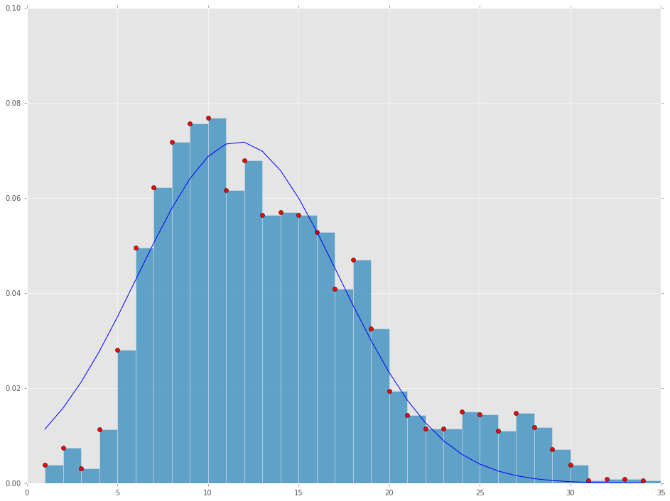
I have a hypothetical y function of x and trying to find/fit a lognormal distribution curve that would shape over the data best. I am using curve_fit function and was able to fit normal distribution, but the curve does not look optimized.

Below are the give y and x data points where y = f(x).

y_axis = [0.00032425299473065838, 0.00063714106162861229, 0.00027009331177605913, 0.00096672396877715144, 0.002388766809835889, 0.0042233337680543182, 0.0053072824980722137, 0.0061291327849408699, 0.0064555344006149871, 0.0065601228278316746, 0.0052574034010282218, 0.0057924488798939255, 0.0048154093097913355, 0.0048619350036057446, 0.0048154093097913355, 0.0045114840997070331, 0.0034906838696562147, 0.0040069911024866456, 0.0027766995669134334, 0.0016595801819374015, 0.0012182145074882836, 0.00098231827111984341, 0.00098231827111984363, 0.0012863691645616997, 0.0012395921040321833, 0.00093554121059032721, 0.0012629806342969417, 0.0010057068013846018, 0.0006081017868837127, 0.00032743942370661445, 4.6777060529516312e-05, 7.0165590794274467e-05, 7.0165590794274467e-05, 4.6777060529516745e-05]

y-axis are probabilities of an event occurring in x-axis time bins:

x_axis = [1.0, 2.0, 3.0, 4.0, 5.0, 6.0, 7.0, 8.0, 9.0, 10.0, 11.0, 12.0, 13.0, 14.0, 15.0, 16.0, 17.0, 18.0, 19.0, 20.0, 21.0, 22.0, 23.0, 24.0, 25.0, 26.0, 27.0, 28.0, 29.0, 30.0, 31.0, 32.0, 33.0, 34.0]

I was able to get a better fit on my data using excel and lognormal approach. When I attempt to use lognormal in python, the fit does not work and I am doing something wrong.

Below is the code I have for fitting a normal distribution, which seems to be the only one that I can fit in python (hard to believe):

#fitting distributino on top of savitzky-golay
%matplotlib inline
import matplotlib
import matplotlib.pyplot as plt
import pandas as pd
import scipy
import scipy.stats
import numpy as np
from scipy.stats import gamma, lognorm, halflogistic, foldcauchy
from scipy.optimize import curve_fit

matplotlib.rcParams['figure.figsize'] = (16.0, 12.0)
matplotlib.style.use('ggplot')
# results from savgol
x_axis = [1.0, 2.0, 3.0, 4.0, 5.0, 6.0, 7.0, 8.0, 9.0, 10.0, 11.0, 12.0,     13.0, 14.0, 15.0, 16.0, 17.0, 18.0, 19.0, 20.0, 21.0, 22.0, 23.0, 24.0, 25.0, 26.0, 27.0, 28.0, 29.0, 30.0, 31.0, 32.0, 33.0, 34.0]
y_axis = [0.00032425299473065838, 0.00063714106162861229, 0.00027009331177605913, 0.00096672396877715144, 0.002388766809835889, 0.0042233337680543182, 0.0053072824980722137, 0.0061291327849408699, 0.0064555344006149871, 0.0065601228278316746, 0.0052574034010282218, 0.0057924488798939255, 0.0048154093097913355, 0.0048619350036057446, 0.0048154093097913355, 0.0045114840997070331, 0.0034906838696562147, 0.0040069911024866456, 0.0027766995669134334, 0.0016595801819374015, 0.0012182145074882836, 0.00098231827111984341, 0.00098231827111984363, 0.0012863691645616997, 0.0012395921040321833, 0.00093554121059032721, 0.0012629806342969417, 0.0010057068013846018, 0.0006081017868837127, 0.00032743942370661445, 4.6777060529516312e-05, 7.0165590794274467e-05, 7.0165590794274467e-05, 4.6777060529516745e-05]

## y_axis values must be normalised
sum_ys = sum(y_axis)

# normalize to 1
y_axis = [_/sum_ys for _ in y_axis]

# def gamma_f(x, a, loc, scale):
#     return gamma.pdf(x, a, loc, scale)

def norm_f(x, loc, scale):
#     print 'loc: ', loc, 'scale: ', scale, "\n"
    return norm.pdf(x, loc, scale)

fitting = norm_f

# param_bounds = ([-np.inf,0,-np.inf],[np.inf,2,np.inf])
result = curve_fit(fitting, x_axis, y_axis)
result_mod = result

# mod scale
# results_adj  = [result_mod[0][0]*.75, result_mod[0][1]*.85]

plt.plot(x_axis, y_axis, 'ro')
plt.bar(x_axis, y_axis, 1, alpha=0.75)
plt.plot(x_axis, [fitting(_, *result[0]) for _ in x_axis], 'b-')
plt.axis([0,35,0,.1])

# convert back into probability
y_norm_fit = [fitting(_, *result[0]) for _ in x_axis]
y_fit = [_*sum_ys for _ in y_norm_fit]
print list(y_fit)

plt.show()

I am trying to get answers two questions:

1. Is this the best fit I will get from normal distribution curve? How can I imporve my the fit?

Normal distribution result:

2. How can I fit a lognormal distribution to this data or is there a better distribution that I can use?

I was playing around with lognormal distribution curve adjust mu and sigma, it looks like that there is possible a better fit. I don't understand what I am doing wrong to get similar results in python.

Smash

Can you show what your fit looks like? – Vasti

Warren: I corrected the negatives, hope that helps. Mikey: I can upload an image of my fit shortly. – Smash

Are your y-values scaled counts? – Pecoraro

Answer 1

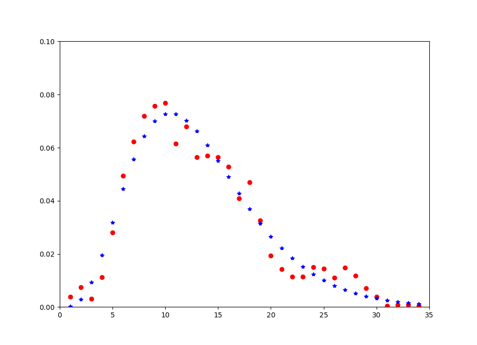
Actually, Gamma distribution might be good fit as @Glen_b proposed. I'm using second definition with \alpha and \beta.

NB: trick I use for a quick fit is to compute mean and variance and for typical two-parametric distribution it is enough to recover parameters and get quick idea if it is good fit or not.

Code

import math
from scipy.misc import comb

import matplotlib.pyplot as plt

y_axis = [0.00032425299473065838, 0.00063714106162861229, 0.00027009331177605913, 0.00096672396877715144, 0.002388766809835889, 0.0042233337680543182, 0.0053072824980722137, 0.0061291327849408699, 0.0064555344006149871, 0.0065601228278316746, 0.0052574034010282218, 0.0057924488798939255, 0.0048154093097913355, 0.0048619350036057446, 0.0048154093097913355, 0.0045114840997070331, 0.0034906838696562147, 0.0040069911024866456, 0.0027766995669134334, 0.0016595801819374015, 0.0012182145074882836, 0.00098231827111984341, 0.00098231827111984363, 0.0012863691645616997, 0.0012395921040321833, 0.00093554121059032721, 0.0012629806342969417, 0.0010057068013846018, 0.0006081017868837127, 0.00032743942370661445, 4.6777060529516312e-05, 7.0165590794274467e-05, 7.0165590794274467e-05, 4.6777060529516745e-05]
x_axis = [1.0, 2.0, 3.0, 4.0, 5.0, 6.0, 7.0, 8.0, 9.0, 10.0, 11.0, 12.0, 13.0, 14.0, 15.0, 16.0, 17.0, 18.0, 19.0, 20.0, 21.0, 22.0, 23.0, 24.0, 25.0, 26.0, 27.0, 28.0, 29.0, 30.0, 31.0, 32.0, 33.0, 34.0]

## y_axis values must be normalised
sum_ys = sum(y_axis)

# normalize to 1
y_axis = [_/sum_ys for _ in y_axis]

m = 0.0
for k in range(0, len(x_axis)):
    m += y_axis[k] * x_axis[k]

v = 0.0
for k in range(0, len(x_axis)):
    t = (x_axis[k] - m)
    v += y_axis[k] * t * t

print(m, v)

b = m/v
a = m * b

print(a, b)

z = []
for k in range(0, len(x_axis)):
    q = b**a * x_axis[k]**(a-1.0) * math.exp( - b*x_axis[k] ) / math.gamma(a)
    z.append(q)

plt.plot(x_axis, y_axis, 'ro')
plt.plot(x_axis, z, 'b*')
plt.axis([0, 35, 0, .1])
plt.show()

Troll

Answer 2

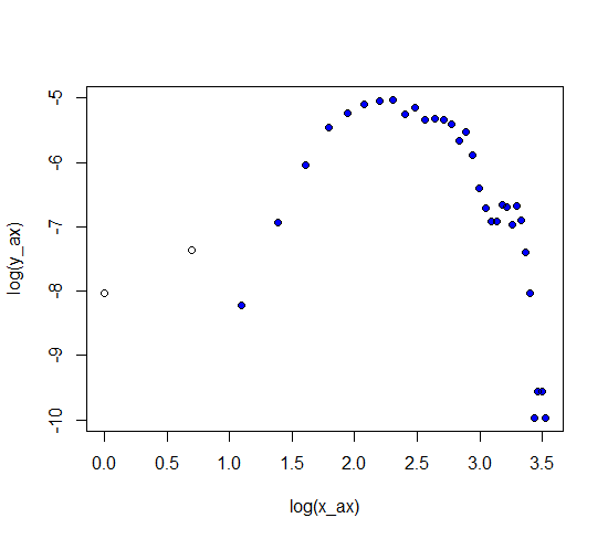
Note that if a lognormal curve is correct and you take logs of both variables, you should have a quadratic relationship; even if that's not a suitable scale for a final model (because of variance effects -- if your variance is near constant on the original scale it will overweight the small values) it should at least give a good starting point for a nonlinear fit.

Indeed aside from the first two points this looks fairly good:

-- a quadratic fit to the solid points would describe that data quite well and should give suitable starting values if you then want to do a nonlinear fit.

(If error in x is at all possible, the lack of fit at the lowest x may be as much issues with error in x as error in y)

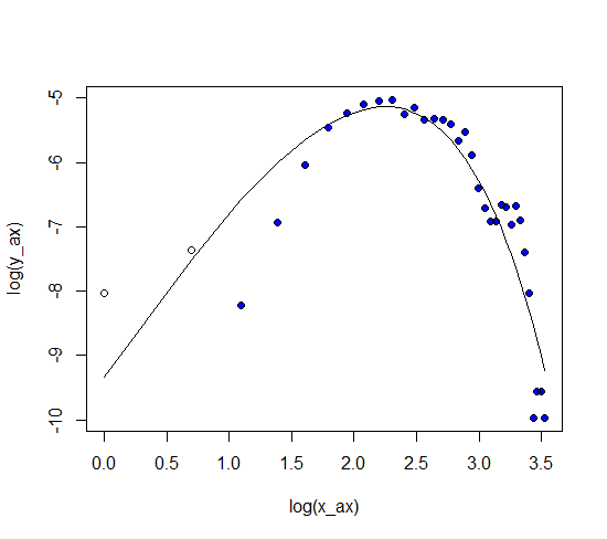
Incidentally, that plot seems to hint that a gamma curve may fit a little better overall than a lognormal one (in particular if you don't want to reduce the impact of those first two points relative to points 4-6). A good initial fit for that can be had by regressing log(y) on x and log(x):

The scaled gamma density is g = c.x^(a-1) exp(-bx) ... taking logs, you get log(g) = log(c) + (a-1) log(x) - b x = b0 + b1 log(x) + b2 x ... so supplying log(x) and x to a linear regression routine will fit that. The same caveats about variance effects apply (so it might be best as a starting point for a nonlinear least squares fit if your relative error in y isn't nearly constant).

Pecoraro

Thanks, this looks promising. I am trying reproduce what you have created and fit gamma, any chance you can paste the code? – Smash

@zad I didn't do that in Python... all I did was regress log(y) on x and log(x) to get the coefficients for a gamma curve (scaled gamma density). If R code would help you, I could paste that but I don't think it will tell you anything useful beyond what I just said in words. The principle is the same in whatever language. – Pecoraro

Answer 3

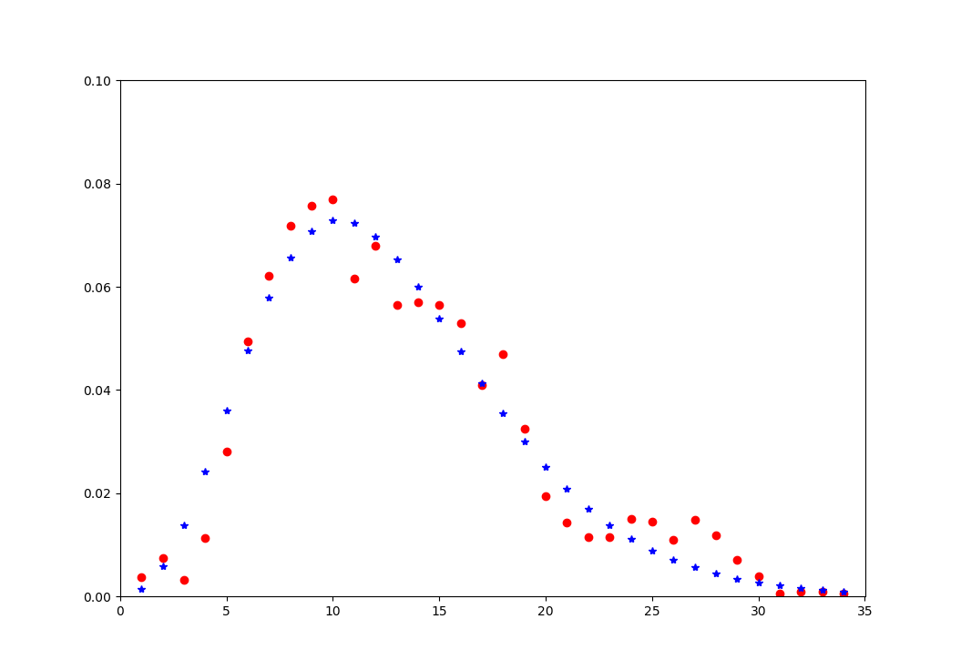
Discrete distribution might look better - your x are all integers after all. You have distribution with variance about 3 times higher than mean, asymmetric - so most likely something like Negative Binomial might work quite well. Here is quick fit

r is a bit above 6, so you might want to move to distribution with real r - Polya distribution.

Code

from scipy.misc import comb

import matplotlib.pyplot as plt

y_axis = [0.00032425299473065838, 0.00063714106162861229, 0.00027009331177605913, 0.00096672396877715144, 0.002388766809835889, 0.0042233337680543182, 0.0053072824980722137, 0.0061291327849408699, 0.0064555344006149871, 0.0065601228278316746, 0.0052574034010282218, 0.0057924488798939255, 0.0048154093097913355, 0.0048619350036057446, 0.0048154093097913355, 0.0045114840997070331, 0.0034906838696562147, 0.0040069911024866456, 0.0027766995669134334, 0.0016595801819374015, 0.0012182145074882836, 0.00098231827111984341, 0.00098231827111984363, 0.0012863691645616997, 0.0012395921040321833, 0.00093554121059032721, 0.0012629806342969417, 0.0010057068013846018, 0.0006081017868837127, 0.00032743942370661445, 4.6777060529516312e-05, 7.0165590794274467e-05, 7.0165590794274467e-05, 4.6777060529516745e-05]
x_axis = [1.0, 2.0, 3.0, 4.0, 5.0, 6.0, 7.0, 8.0, 9.0, 10.0, 11.0, 12.0, 13.0, 14.0, 15.0, 16.0, 17.0, 18.0, 19.0, 20.0, 21.0, 22.0, 23.0, 24.0, 25.0, 26.0, 27.0, 28.0, 29.0, 30.0, 31.0, 32.0, 33.0, 34.0]

## y_axis values must be normalised
sum_ys = sum(y_axis)

# normalize to 1
y_axis = [_/sum_ys for _ in y_axis]

s = 1.0 # shift by 1 to have them all at 0
m = 0.0
for k in range(0, len(x_axis)):
    m += y_axis[k] * (x_axis[k] - s)

v = 0.0
for k in range(0, len(x_axis)):
    t = (x_axis[k] - s - m)
    v += y_axis[k] * t * t

print(m, v)

p = 1.0 - m/v
r = int(m*(1.0 - p) / p)

print(p, r)

z = []
for k in range(0, len(x_axis)):
    q = comb(k + r - 1, k) * (1.0 - p)**r * p**k
    z.append(q)

plt.plot(x_axis, y_axis, 'ro')
plt.plot(x_axis, z, 'b*')
plt.axis([0, 35, 0, .1])
plt.show()

Troll

Answer 4

In Python, I explained a trick here of how to fit a LogNormal very simply using OpenTURNS library:

import openturns as ot

n_times = [int(y_axis[i] * N) for i in range(len(y_axis))]
S = np.repeat(x_axis, n_times)

sample = ot.Sample([[p] for p in S])
fitdist = ot.LogNormalFactory().buildAsLogNormal(sample)

That's it!

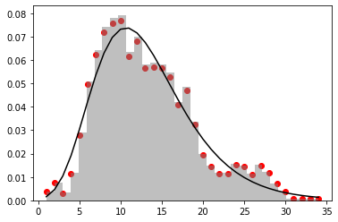
print(fitdist) will show you >>> LogNormal(muLog = 2.92142, sigmaLog = 0.305, gamma = -6.24996)

and the fitting seems good:

import matplotlib.pyplot as plt

plt.hist(S, density =True, color = 'grey', bins = 34, alpha = 0.5)
plt.scatter(x_axis, y_axis, color= 'red')
plt.plot(x_axis, fitdist.computePDF(ot.Sample([[p] for p in x_axis])), color = 'black')
plt.show()

Xuthus