Flatten or detrend a seasonal time series

Question

I have a repeating time series with a seasonal (weekly) pattern, and I'd like to return the same time series with no week-over-week trend, taking the first value as a starting point.

To be specific, the 1st value will still be 39.8, but the 8th value will also be 39.8 rather than 17.1. If the first seven values were just repeated then there would be a week-long negative trend repeated and I'd like to have no trend at all (so the 7th value of 6.2 would also be higher).

Is there an elegant way to do this, especially one that is robust to zero-valued entries in a time-series (I have a lot of them)?

We can assume the time series trend is linear and constant (i.e. not just piecewise linear).

demand <- ts(
  c(39.8, 33.5, 40.6, 23.6, 11.9, 12.3, 6.2, 17.1, 10.8, 18, 1, -10.7, 
-10.4, -16.5, -5.6, -11.9, -4.7, -21.7, -33.4, -33.1, -39.2, -28.2, 
-34.6, -27.4, -44.4, -56.1, -55.7, -61.8, -50.9, -57.2, -50.1),
frequency = 7
)

plot(demand)

Floccus

Answer 1

You can do something like this:

trend = stl(demand, s.window = "periodic")$time.series[,2]

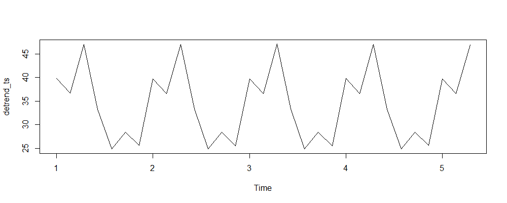
detrend_ts = demand - (trend - trend[1])

plot(detrend_ts)

Result:

> detrend_ts
Time Series:
Start = c(1, 1) 
End = c(5, 3) 
Frequency = 7 
 [1] 39.80000 36.72792 47.05584 33.28224 24.80864 28.43514 25.56165 39.69889 36.63614
[10] 47.08241 33.32868 24.86478 28.40088 25.53956 39.67825 36.63383 47.08942 33.32204
[19] 24.85466 28.38747 25.52029 39.76777 36.61526 47.05556 33.29586 24.82129 28.44673
[28] 25.57045 39.69417 36.61948 46.94480

Notes:

Basically, I used STL decomposition (Seasonal Decomposition of Time Series by Loess) to estimate the trend, then subtracted it from demand. Since you wanted the de-trended time series to start at 39.8, I also subtracted the first value of the trend from trend.

Grandfather

Answer 2

As the trend is linear, you can also use a linear fit

linear_fit <- lm(demand ~ time(demand))
plot(demand - linear_fit$fitted.values + linear_fit$fitted.values[1],
    ylab = "detrended demand", typ = 'o')

Function decompose is also helpful to obtain the trend. As it applies a centered moving average, the trend will have 3 NA at the beginning of the series and 3 at the end.

demand_decomposed <- decompose(demand)
plot(demand - demand_decomposed$trend, ylab = 'detrended demand', typ = 'o')

Note that the trend can be computed directly using filter function to get the moving average used by decompose function

trend_ma <- filter(demand, rep(1/7, 7), method = "convolution", sides = 2) 
plot(demand - trend_ma, typ = 'o', ylab = "detrended demand")

The last two plots were not adjusted to the trend value at time 1 as it does not exist. It is possible to replace NA for the value it should have according to the the seasonal pattern:

seasonal <- demand - trend_ma
na_values_time_in_period <- cycle(demand)[is.na(seasonal)]
value_time_in_period <- tapply(seasonal, cycle(demand), mean, na.rm = TRUE)
seasonal[is.na(seasonal)] <- value_time_in_period[na_values_time_in_period]

Loan