Aligning maps made using basemap

Question

Is there a way to align python basemaps like this figure below?

Here's some sample basemap code to produce a map:

from mpl_toolkits.basemap import Basemap
import matplotlib.pyplot as plt

fig = plt.figure(figsize=(8, 4.5))
plt.subplots_adjust(left=0.02, right=0.98, top=0.98, bottom=0.00)
m = Basemap(projection='robin',lon_0=0,resolution='c')
m.fillcontinents(color='gray',lake_color='white')
m.drawcoastlines()
plt.savefig('world.png',dpi=75)

Cancel

Could you be a bit more specific? If you just want several Basemaps in one figure, use subplots. If that is not what you are after, you need to tell us more about your actual problem. – Copenhagen

thanks @ThomasKühn, I want several basemaps in one figure but more importantly, I want to align them at an angle (somewhat similar to the figure in the question). – Cancel

Answer 1

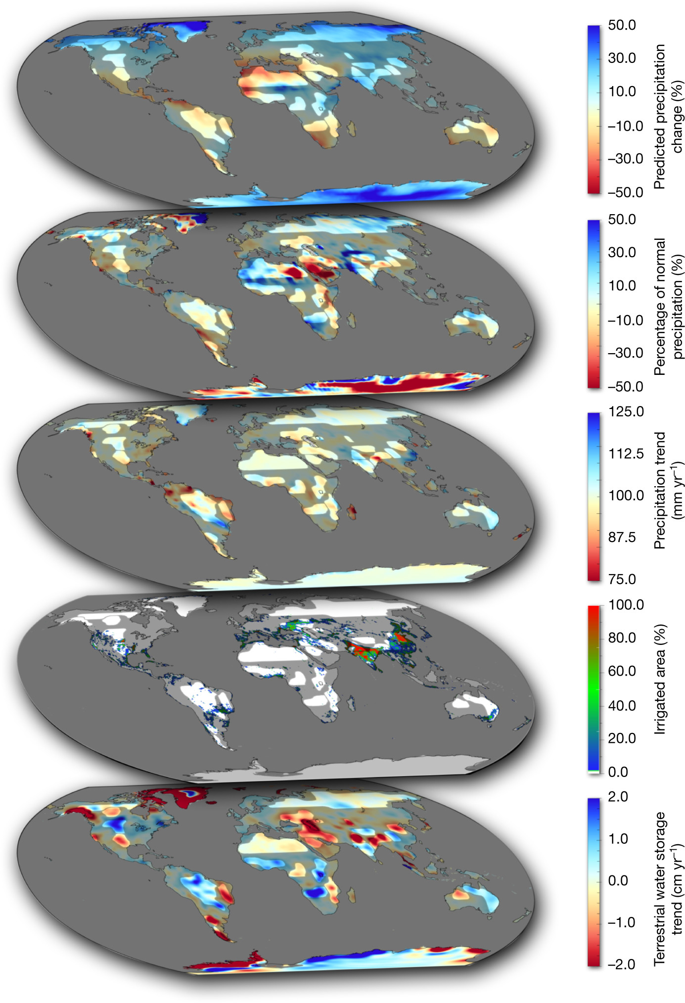
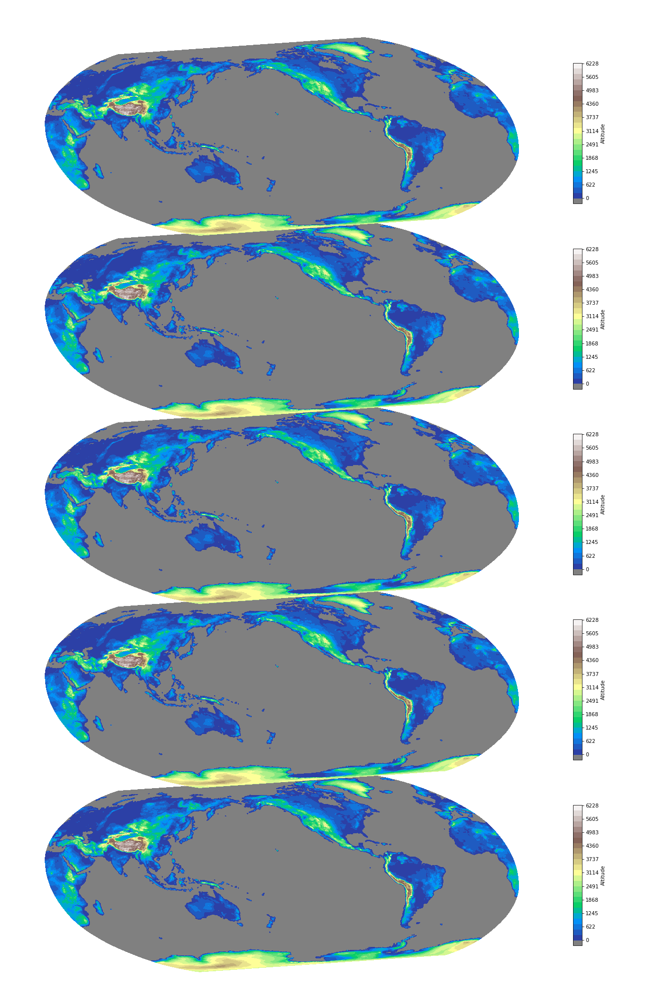
I am not an expert with Matplotlib, but I found a way to get a similar result by using the data files included in the source folder of basemap. They can be combined into a meshgrid to plot some data, in the example below we plot the altitude at every point.

One of the tricks I used is to set matplotlib to an orthogonal projection so that there is no distortion in the vertical spacing of the maps.

I have put the parameters at the beginning of the code as you may find it useful to adjust.

One thing I couldn't get my head around is the shadow under the maps.

from mpl_toolkits.mplot3d import proj3d
from mpl_toolkits.basemap import Basemap
from mpl_toolkits.axes_grid1.inset_locator import inset_axes
import numpy as np
import matplotlib.pyplot as plt

# Parameters
n_maps = 5 # Number of maps
z_spacing = 4. # Spacing of maps along z
z_reduction = 1E-8 # Reduction factor for Z data, makes the map look flat
view_angles = (14., -100.) # Set view port angles
colbar_bottom = 0.2 # Space at the bottom of colorbar column
colbar_spacing = .132 # Space between colorbars
colbar_height = 0.1 # Height of colorbars

# Set orthogonal projection
def orthogonal_proj(zfront, zback):
    a = (zfront+zback)/(zfront-zback)
    b = -2*(zfront*zback)/(zfront-zback)
    return np.array([[1,0,0,0],
                     [0,1,0,0],
                     [0,0,a,b],
                     [0,0,-0.0001,zback]])

proj3d.persp_transformation = orthogonal_proj

fig = plt.figure(figsize=[30, 10*n_maps])
ax = fig.gca(projection='3d')

etopo = np.loadtxt('etopo20data.gz')
lons  = np.loadtxt('etopo20lons.gz')
lats  = np.loadtxt('etopo20lats.gz')
# Create Basemap instance for Robinson projection.
m = Basemap(projection='robin', lon_0=0.5*(lons[0]+lons[-1]))
# Compute map projection coordinates for lat/lon grid.
X, Y = m(*np.meshgrid(lons,lats))

# Exclude the oceans
Z = etopo.clip(-1)

# Set the colormap
cmap = plt.cm.get_cmap("terrain")
cmap.set_under("grey")

for i in range(n_maps):
    c = ax.contourf(X, Y, z_spacing*i + z_reduction*Z, 30, cmap=cmap, vmin=z_spacing*i, extend='neither')
    cax = inset_axes(ax,
               width="5%",
               height="100%",
               loc=3,
               bbox_to_anchor=(.85, colbar_spacing*i+colbar_bottom, .2, colbar_height),
               bbox_transform=ax.transAxes,
               borderpad=0
               )
    cb = fig.colorbar(c, cax=cax)
    cb.set_label("Altitude")
    # Reset the ticks of the color bar to match initial data
    cb.set_ticks([z_spacing * i + j/10. * z_reduction * Z.max() for j in range(11)])
    cb.set_ticklabels([str(int(j/10. * Z.max())) for j in range(11)])

ax.set_axis_off()
ax.view_init(*view_angles)
ax.set_xlim3d(X.min(), X.max())
ax.set_ylim3d(Y.min(), Y.max())
ax.set_zlim3d(-1E-2, (n_maps-1)*z_spacing)

plt.savefig('world.png',dpi=75)

Edit:

If you want shadows and don't mind the extra compute time you can change the beginning of the for loop with something along the lines of:

shadow_Z = np.empty(Z.shape)
for i in range(n_maps):
    c = ax.contourf(X, Y, z_spacing*i + z_reduction*Z, 30, cmap=cmaps[i], vmin=z_spacing*i, extend='neither')
    for j in range(10):
        shadow_Z.fill(z_spacing*i - 1E-2 * j)
        s = ax.contourf((X - X.mean()) * (1 + 8E-3 * j) + X.mean() + 2E5, 
                        (Y - Y.mean()) * (1 + 8E-3 * j) + Y.mean() - 2E5, 
                        shadow_Z, colors='black', alpha=0.1 - j * 1E-2)

Knisley

@Cancel I managed to get some shadows under the maps although it's a bit slow. – Knisley

thanks @jacques! this soln goes above and beyond what I expected – Cancel

could you also upload the .gz files somehwere? – Cancel

You can get the .gz files in the examples folder of the sources: sourceforge.net/projects/matplotlib/files/matplotlib-toolkits/… – Knisley