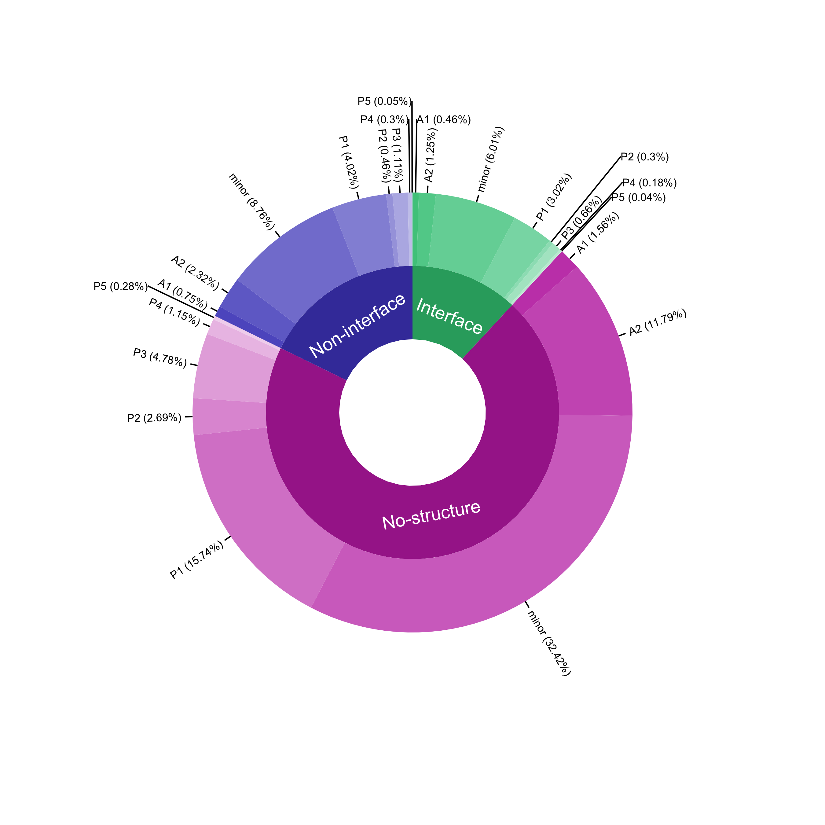
PieDonut does not display some pie labels

Question

I've used the following data to plot the circular plot from the picture below and I can't display the labels of the narrowest sections. Any clue why?. I've tried reducing the size of the label and doesn't work.

data

      level1    level2             size
      Interface     A1           191730
      Interface     A2           524340
      Interface  minor          2529189
      Interface     P1          1273072
      Interface     P2           126295
      Interface     P3           279050
      Interface     P4            74326
      Interface     P5            16646
   No structure     A1 654914.333333333
  No structure     A2 4965368.33333333
  No structure  minor 13654304.3333333
  No structure     P1 6627555.33333333
  No structure     P2          1131774
  No structure     P3          2011299
  No structure     P4           485273
  No structure     P5           116248
 Non-interface     A1           317491
 Non-interface     A2           978807
 Non-interface  minor          3689632
 Non-interface     P1          1690987
 Non-interface     P2           192730
 Non-interface     P3           468848
 Non-interface     P4           125529
 Non-interface     P5            21676

code:

#create PieDonut
require(ggplot2)
require(moonBook)
require(webr)
PieDonut(data,
         aes(pies= level2, donuts = level1, count = size),
         ratioByGroup=T,
         addDonutLabel = F,
         labelpositionThreshold = 0.4,
         donutLabelSize = 3,
         use.labels = F,
         title="Title",
         maxx = 1.5,
         r0=0,showPieName=FALSE)

Result:

Note: As a workaround, I used the sunburst package. However I think it looks very confusing, that's why I want to use the other plot. Nevertheless, here's my piece of code and the plot.

# install ggsunburst
if (!require("ggplot2")) install.packages("ggplot2")
if (!require("rPython")) install.packages("rPython")
install.packages("http://genome.crg.es/~didac/ggsunburst/ggsunburst_0.0.10.tar.gz", repos=NULL, type="source")
library(ggsunburst)
library(ggrepel)

names(data) = c("parent","node", "size")
data$location <- data$parent
write.table(data, file = 'data.csv', row.names = F, sep = ",")
sb <- sunburst_data('data.csv', type = 'node_parent', sep = ",", node_attributes = c("location","size"))
sb$rects[!sb$rects$leaf,]$location <- sb$rects[!sb$rects$leaf,]$name
colors= c("#2DA86D", "#A72D98", "#423FA9", "#4BC88B", "#5FCE98", "#73D4A5", "#87DAB2", "#9BE0BF", "#AFE6CB", "#C3ECD8", "#D7F2E5",
  "#C74BB7", "#CD5FBF", "#D373C7", "#D987CF", "#E09BD7", "#E6AFDF", "#ECC3E7", "#F2D7EF", "#5F5DC8", "#716FCE", "#8381D4", "#9493DA", "#A6A5E0", "#B8B7E6", "#C9C9EC", "#DBDBF2")

n_total_size = 42115268

p <- ggsunburst::sunburst(sb,
              rects.fill = colors,
              rects.fill.aes=0,
              rects.size =2,
              node_labels.size = 5,
              leaf_labels.size = 3,
              blank = T,
              leaf_labels = T,
              rects.color = "white",
              node_labels = T,
              node_labels.color = "white",
              node_labels.min = 0)+
  geom_label_repel(data = sb$leaf_labels,
                   aes(x=x,
                       y=0,
                       label=paste(round(size/n_total_size * 100, 2), '%')),
              colour = colors[4:27],
              nudge_y = .55, 
              segment.size = 0.7, 
              show.legend = T,
              segment.colour = "black",
              fontface = 'bold')

Hyperemia

You probably need to include the library you've used, to enable us to follow you. – Odell

Try also the showRatioThreshold argument in PieDonut(). It sets the minimum threshold of label sizes based on ratio – Operation

Answer 1

Explicitly setting the PieDonut parameter showRatioThreshold = F did the trick for me.

Sedillo

Answer 2

kudos for using ggrepel with ggsunburst, however I agree the result could be improved.

It is not the ideal solution, but you can plot separately those labels with smaller size. You can split sb$leaf_labels based on size, and manually set a new_y

library(ggsunburst)

data <- read.table(header = T, text = "
level1    level2             size
Interface     A1           191730
Interface     A2           524340
Interface  minor          2529189
Interface     P1          1273072
Interface     P2           126295
Interface     P3           279050
Interface     P4            74326
Interface     P5            16646
No-structure     A1 654914.333333333
No-structure     A2 4965368.33333333
No-structure  minor 13654304.3333333
No-structure     P1 6627555.33333333
No-structure     P2          1131774
No-structure     P3          2011299
No-structure     P4           485273
No-structure     P5           116248
Non-interface     A1           317491
Non-interface     A2           978807
Non-interface  minor          3689632
Non-interface     P1          1690987
Non-interface     P2           192730
Non-interface     P3           468848
Non-interface     P4           125529
Non-interface     P5            21676")

names(data) = c("parent","node", "size")
data$location <- data$parent
write.table(data, file = 'data.csv', row.names = F, sep = ",")
sb <- sunburst_data('data.csv', type = 'node_parent', sep = ",", node_attributes = c("location","size"))
sb$rects[!sb$rects$leaf,]$location <- sb$rects[!sb$rects$leaf,]$name
colors= c("#2DA86D", "#A72D98", "#423FA9", "#4BC88B", "#5FCE98", "#73D4A5", "#87DAB2", "#9BE0BF", "#AFE6CB", "#C3ECD8", "#D7F2E5",
          "#C74BB7", "#CD5FBF", "#D373C7", "#D987CF", "#E09BD7", "#E6AFDF", "#ECC3E7", "#F2D7EF", "#5F5DC8", "#716FCE", "#8381D4", "#9493DA", "#A6A5E0", "#B8B7E6", "#C9C9EC", "#DBDBF2")

n_total_size = 42115268

sb$leaf_labels <- within(sb$leaf_labels,{
  percentage = paste("(",round(size/n_total_size * 100, 2),"%)",sep = "")
  new_label = paste(label,percentage, sep = " ")
  })

text_size <- 3
wide <- subset(sb$leaf_labels, size > 191730.0)
narrow <- subset(sb$leaf_labels, size <= 191730.0)
narrow$new_y <- c(1, 1.25, 1, .75, 1, 1, 1.25)

ggsunburst::sunburst(sb,
                          rects.fill = colors,
                          rects.fill.aes=0,
                          rects.size =0,
                          node_labels.size = 5,
                          leaf_labels.size = 3,
                          blank = T,
                          leaf_labels = F,
                          rects.color = "white",
                          node_labels = T,
                          node_labels.color = "white",
                          node_labels.min = 0
                          ) + 

  geom_segment(data = wide, aes(x=x, xend=x, y=y_out, yend=.1), size = .5) +
  geom_segment(data = narrow, aes(x=x, xend=x, y=y_out, yend=new_y), size = .5) +
  geom_text(data = wide, aes(x=x, y=.15, label=new_label, angle=angle, hjust=hjust), size = text_size) +
  geom_text(data = narrow, aes(x=x, y=new_y, label=new_label, angle=0, hjust=hjust), size = text_size) 

Protuberancy