Small multiple maps with geom_sf at the same spatial scale
Asked Answered
T

3

6

I would like to plot a figure with small multiple maps using ggplot2::geom_sf. The challenge here is how to do this keeping all maps centered in the image and at the same spatial scale. Here is the problem (data for reproducible example below):

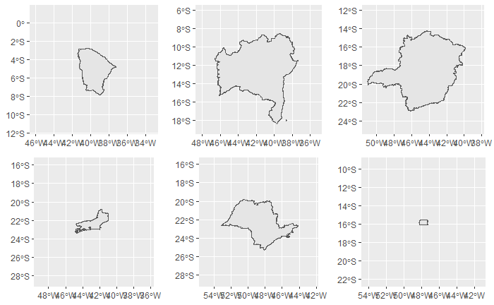
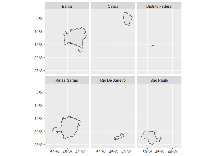
A simple map using facet_wrap put all polygons at the same spatial scale, but they are not centered.

ggplot(states6) +
  geom_sf() +
  facet_wrap(~name_state)

enter image description here

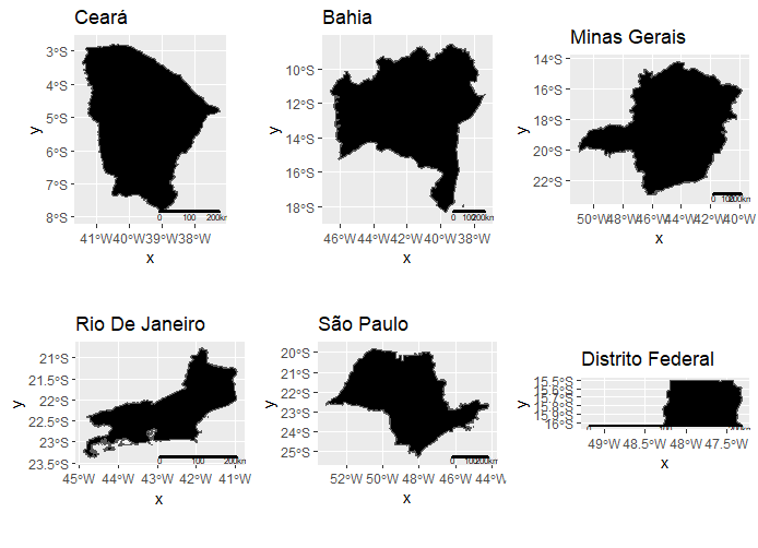
Here is a solution from this SO question that uses cowplot. In this case, polygons are centered but they come at different spatial scales

g <- purrr::map(unique(states6$name_state),
                function(x) {

                  # subset data
                  temp_sf <- subset(states6, name_state == x)

                  ggplot() +
                    geom_sf(data = temp_sf, fill='black') +
                    guides(fill = FALSE) +
                    ggtitle(x) +
                    ggsn::scalebar(temp_sf, dist = 100, st.size=2, 
                                   height=0.01, model = 'WGS84', 
                                   transform = T, dist_unit='km') 
                    })

g2 <- cowplot::plot_grid(plotlist = g)
g2

enter image description here

I've found the same problem using the tmaplibrary.

 tm_shape(states6) +
   tm_borders(col='black') +
   tm_fill(col='black') +
   tm_facets(by = "name_state ", ncol=3) +
   tm_scale_bar(breaks = c(0, 50, 100), text.size = 3)

Desired output

The output I would like to get is something similar to this:

enter image description here

Data for reproducible example

library(sf)
library(geobr)
library(mapview)
library(ggplot2)
library(ggsn)
library(cowplot)
library(purrr)
library(tmap)

# Read all Brazilian states
states <- geobr::read_state(code_state = 'all', year=2015)

# Select six states
states6 <- subset(states, code_state %in% c(35,33,53,29,31,23))
Trapshooting answered 24/10, 2019 at 22:22 Comment(2)
Can you specify what you desire? How we can plot on the same scale but keep different objects centered anyway is unclear to me.Selfexpression
I've added an image to illustrate the desired outputTrapshooting
C
4

It´s not ideal but you can make several plots programmatically with the same box size and then put them together using ::gridExtra. To get the center of each box, use the centroid of each geometry.

library(sf)
library(geobr)
library(mapview)
library(ggplot2)
library(gridExtra)

Read all Brazilian states:

states <- geobr::read_state(code_state = 'all', year=2015)

Select six states:

states6 <- subset(states, code_state %in% c(35,33,53,29,31,23))

centroids, for reference in the ggplot bellow (I had to set the projection, make changes here if needed):

states6$centroid <- 
     sf::st_transform(states6, 29101) %>% 
     sf::st_centroid() %>% 
     sf::st_transform(., '+proj=longlat +ellps=GRS80 +no_defs')  %>% 
     sf::st_geometry()

set padding:

padding <-7 

function to make plots:

graph <- function(x){
  ggplot2::ggplot(states6[x,]) +
           geom_sf() +
           coord_sf(xlim = c(states6$centroid[[x]][1]-padding , 
                             states6$centroid[[x]][1]+padding), 
                    ylim = c(states6$centroid[[x]][2]-padding , 
                             states6$centroid[[x]][2]+padding), 
                    expand = FALSE)
}

create a bunch of plots:

plot_list <- lapply(X = 1:nrow(states6), FUN = graph)

grid them together:

g <- cowplot::plot_grid(plotlist = plot_list, ncol = 3)
g

results

Carnatic answered 25/10, 2019 at 2:10 Comment(0)
L
3

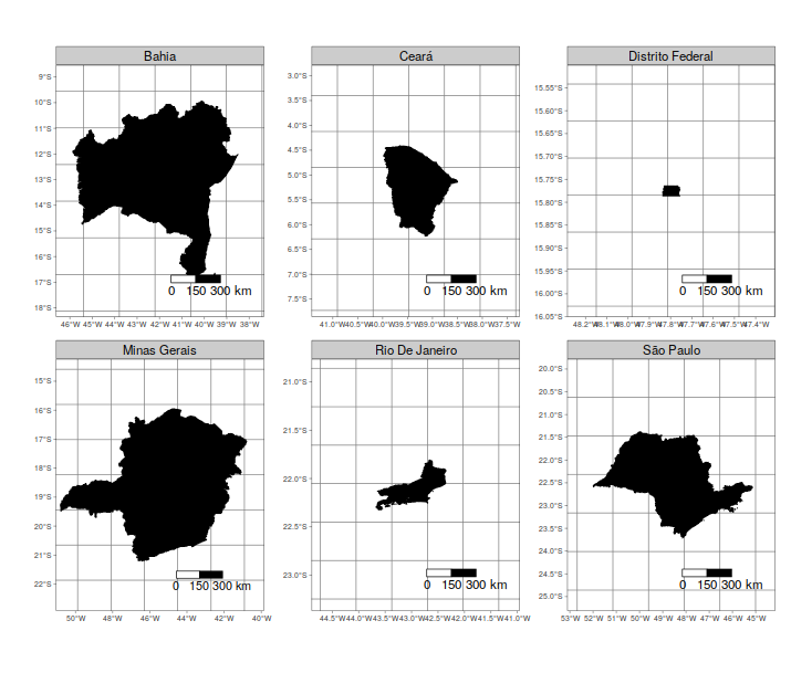
A bit of a hack, but here is a possible tmap solution based on computing the max width of the different states and then create a "dummy" layer of points spaced max_width/2 from the centroids of each state to "force" a constant width of the facets and thus a constant scale:

library(sf)
library(geobr)
library(tmap)
library(dplyr)

# Read all Brazilian states
states <- geobr::read_state(code_state = 'all', year=2015)

# Select six states
states6 <- subset(states, code_state %in% c(35,33,53,29,31,23)) %>% 
    sf::st_set_crs(4326)

# compute bboxes and find width of the widest one
bboxes <- lapply(sf::st_geometry(states6), 
                 FUN = function(x) as.numeric(st_bbox((x))))
which_max_wid <- which.max(lapply(bbs, FUN = function(x) abs(x[1] - x[3])))              
max_wid <- bbs[[which_max_wid]][1] - bbs[[which_max_wid]][3]

# create some fake points, at a distance of max_wid/2 from 
# centroids of each state, then a multipoint by state_name

fake_points_min <- st_sf(name_state = states6$name_state, 
                         geometry = st_geometry(sf::st_centroid(states6)) - c(max_wid/2, 0))
fake_points_max <- st_sf(name_state = states6$name_state, 
                         geometry = st_geometry(sf::st_centroid(states6)) + c(max_wid/2, 0))

fake_points <- rbind(fake_points_min,fake_points_max) %>% 
    dplyr::group_by(name_state) %>% 
    dplyr::summarize() %>% 
    dplyr::ungroup() %>% 
    sf::st_set_crs(4326)

# plot
plot <- tm_shape(states6) +
    tm_graticules() +
    tm_borders(col='black') +
    tm_fill(col='black') +
    tm_facets(by = "name_state", ncol=3) +
    tm_scale_bar(breaks = c(0, 150, 300), text.size = 3) + 
    tm_shape(fake_points)  +  #here we add the point layer to force constant width!
    tm_dots(alpha = 0)+ 
    tm_facets(by = "name_state", ncol=3)
plot

, giving:

enter image description here

Limy answered 25/10, 2019 at 15:42 Comment(0)
K
1

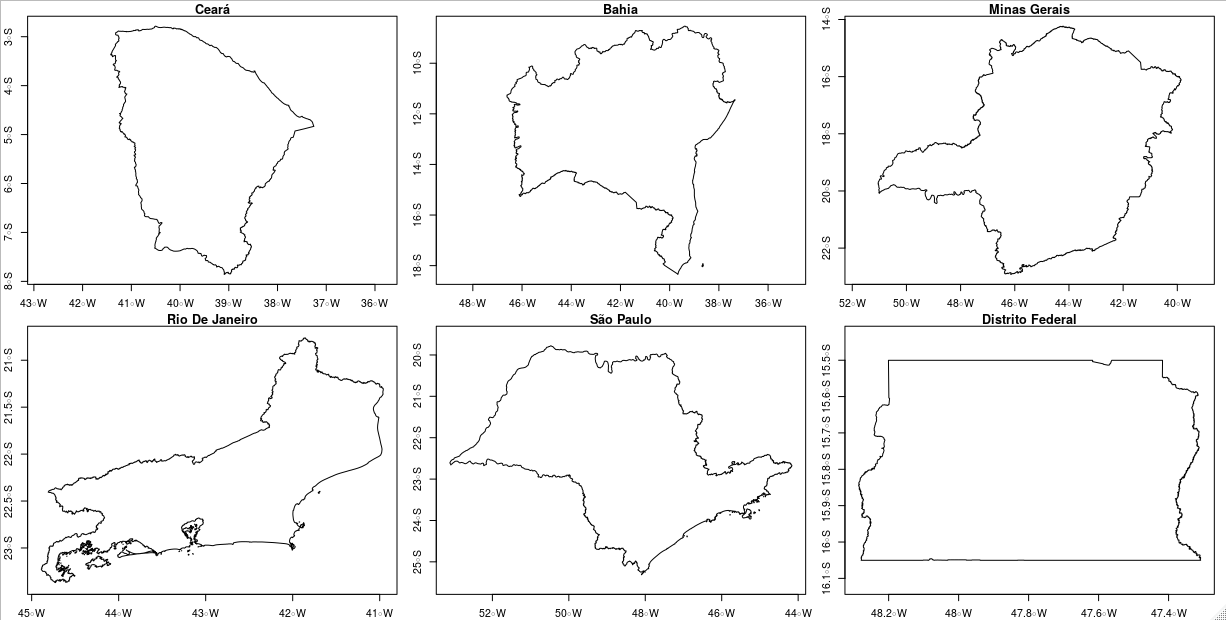
Most of the times I prefer plot for sf

library(sf)
library(geobr)

# Read all Brazilian states
states <- geobr::read_state(code_state = 'all', year=2015)

# Select six states
states6 <- subset(states, code_state %in% c(35,33,53,29,31,23))
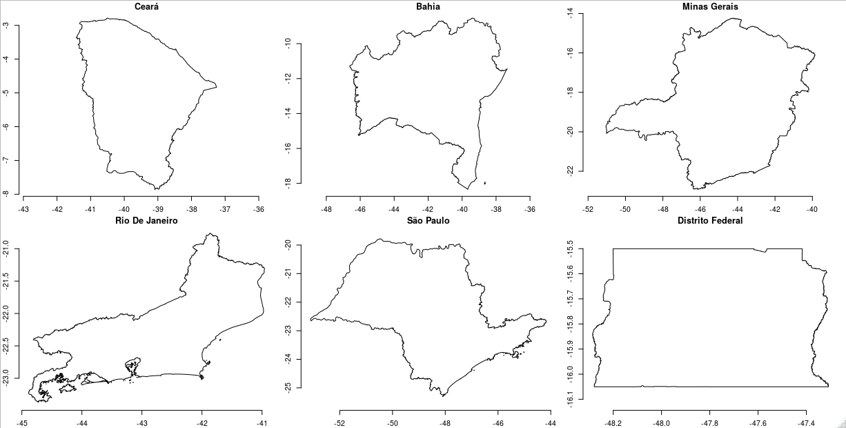
par(mfrow = c(2, 3))
for(i in 1:nrow(states6)){
  plot(states6$geometry[i], axes = T, main = states6$name_state[i])  
}
par(mfrow = c(1,1))

enter image description here

However, removing the axis can be also effective

par(mfrow = c(2, 3))
for(i in 1:nrow(states6)){
  plot(states6$geometry[i], axes = F, main = states6$name_state[i])  
  axis(1)
  axis(2)
}
par(mfrow = c(1,1))

enter image description here

As probably you would want to add a background, add the option reset = FALSE as explained here and you can add several other sf or stars objects

EDIT1: You could also try imagemagick

library(ggplot2)
imas <- paste0(letters[1:6], ".png")
for(i in 1:nrow(states6)) {
png( imas[i])
  print(
    ggplot(states6[i,]) +
      geom_sf()  +
      ggtitle(states6$name_state[i])
)  
  dev.off()
}

library(magick)
a <- image_append(image = c(image_read(imas[1]), 
                       image_read(imas[2]),
                       image_read(imas[3])))


b <- image_append(image = c(image_read(imas[4]), 
                            image_read(imas[5]),
                            image_read(imas[6])))

image_append(c(a,b), stack = T)

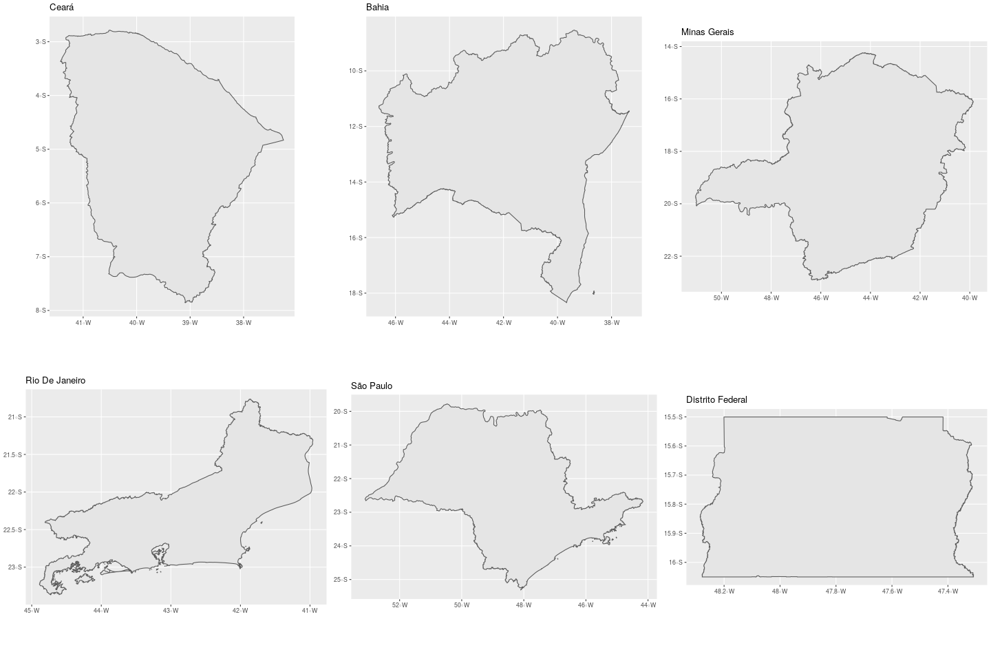
enter image description here

Kwapong answered 25/10, 2019 at 19:21 Comment(2)
Hi Sergio. Thanks for the suggestions. A key challenge here is to keep all maps at the same spatial scale.Trapshooting
I see, sorry, i did not read that part. However, as Brazil is a really big country, I think it is difficult to keep the same scaleKwapong

© 2022 - 2024 — McMap. All rights reserved.