Why does scipy.optimize.minimize (default) report success without moving with Skyfield?

Question

scipy.optimize.minimize using default method is returning the initial value as the result, without any error or warning messages. While using the Nelder-Mead method as suggested by this answer solves the problem, I would like to understand:

Why does the default method returns the wrong answer without warning the starting point as the answer - and is there a way I can protect against "wrong answer without warning" avoid this behavior in this case?

Note, the function separation uses the python package Skyfield to generate the values to be minimized which is not guaranteed smooth, which may be why Simplex is better here.

RESULTS:

test result: [ 2.14159739] 'correct': 2.14159265359 initial: 0.0

default result: [ 10000.] 'correct': 13054 initial: 10000

Nelder-Mead result: [ 13053.81011963] 'correct': 13054 initial: 10000

FULL OUTPUT using DEFAULT METHOD:
   status: 0
  success: True
     njev: 1
     nfev: 3
 hess_inv: array([[1]])
      fun: 1694.98753895812
        x: array([ 10000.])
  message: 'Optimization terminated successfully.'
      jac: array([ 0.])
      nit: 0

FULL OUTPUT using Nelder-Mead METHOD:
  status: 0
    nfev: 63
 success: True
     fun: 3.2179306044608054
       x: array([ 13053.81011963])
 message: 'Optimization terminated successfully.'
     nit: 28

Here is the full script:

def g(x, a, b):
    return np.cos(a*x + b)

def separation(seconds, lat, lon):
    lat, lon, seconds = float(lat), float(lon), float(seconds) # necessary it seems
    place = earth.topos(lat, lon)
    jd = JulianDate(utc=(2016, 3, 9, 0, 0, seconds))
    mpos = place.at(jd).observe(moon).apparent().position.km
    spos = place.at(jd).observe(sun).apparent().position.km
    mlen = np.sqrt((mpos**2).sum())
    slen = np.sqrt((spos**2).sum())
    sepa = ((3600.*180./np.pi) *
            np.arccos(np.dot(mpos, spos)/(mlen*slen)))
    return sepa

from skyfield.api import load, now, JulianDate
import numpy as np
from scipy.optimize import minimize

data = load('de421.bsp')

sun   = data['sun']
earth = data['earth']
moon  = data['moon']

x_init = 0.0
out_g = minimize(g, x_init, args=(1, 1))
print "test result: ", out_g.x, "'correct': ", np.pi-1, "initial: ", x_init    # gives right answer

sec_init = 10000
out_s_def = minimize(separation, sec_init, args=(32.5, 215.1))
print "default result: ", out_s_def.x, "'correct': ", 13054, "initial: ", sec_init

sec_init = 10000
out_s_NM = minimize(separation, sec_init, args=(32.5, 215.1),
                 method = "Nelder-Mead")
print "Nelder-Mead result: ", out_s_NM.x, "'correct': ", 13054, "initial: ", sec_init

print ""
print "FULL OUTPUT using DEFAULT METHOD:"
print out_s_def
print ""
print "FULL OUTPUT using Nelder-Mead METHOD:"
print out_s_NM

Goody

Here is a related Skyfield question. – Goody

oh sorry, missed that. I guess the problem is that minimize per default uses an algorithms that requires your function to be smooth. If your function is not smooth, you end up in a garbage-in-garbage-out situation. – Corbitt

I don't understand what you are asking then. The default algorithm is simply not suited for your problem if your function can be non-smooth. Why do you want to use it then? Are you asking how to find out if the function is smooth? – Corbitt

Once again the answer is already there and it's pretty clear: "Why does the default method returns the wrong answer without warning - and is there a way I can protect against 'wrong answer without warning' behavior in this case?" – Goody

The documentation states that the (default) "BFGS has proven good performance even for non-smooth optimizations". Perhaps the documentation should be updated to more clearly suggest using a different solver for non-smooth problems? – Noguchi

There are different kinds of non-smoothness, so it may be it works OK for other problems. But it's probably not good general advice to suggest derivative-based optimizers when derivatives don't exist (at crucial points). – Machiavelli

Answer 1

1)

Your function is piecewise constant (has small-scale "staircase" pattern). It is not everywhere differentiable.

The gradient of the function at the initial guess is zero.

The default BFGS optimizer sees the zero gradient and decides it is a local minimum by its criteria (which are based on assumptions about the input function that are not true in this case, such as differentiability).

Basically, the exactly flat regions bomb the optimizer. The optimizer probes the function in the small exactly flat region around the initial point, where everything looks like the function is just a constant, so it thinks you gave it a constant function. Because your function is not differentiable everywhere, it is possible that almost all initial points are inside such flat regions, so that this can happen without bad luck in the choice of the initial point.

Note also that Nelder-Mead is not immune to this --- it just happens its initial simplex is larger than the size of the staircase, so it probes the function around a larger spot. If the initial simplex would be smaller than the staircase size, the optimizer would behave similarly as BFGS.

2)

General answer: local optimizers return local optima. Whether these coincide with the true optimum depends on the properties of the function.

In general, to see if you're stuck in a local optimum, try different initial guesses.

Also, using a derivative-based optimizer on a non-differentiable function is not a good idea. If the function is differentiable on a "large" scale, you can adjust the step size of the numerical differentiation.

Because there is no cheap/general way to check numerically if a function is everywhere differentiable, no such check is done --- instead it is an assumption in the optimization method that must be ensured by whoever inputs the objective function and chooses the optimization method.

Machiavelli

OK that's exactly what I needed to understand! Thank you for taking the time to explain clearly what's going on. I've added a plot in a "supplemental" answer showing that below a 1E-03 seconds even the JulianDate is discrete. That's fine for most uses of the package but of course not for derivatives. – Goody

I've changed the title and removed the word "fail" since this is exactly what is expected. – Goody

Answer 2

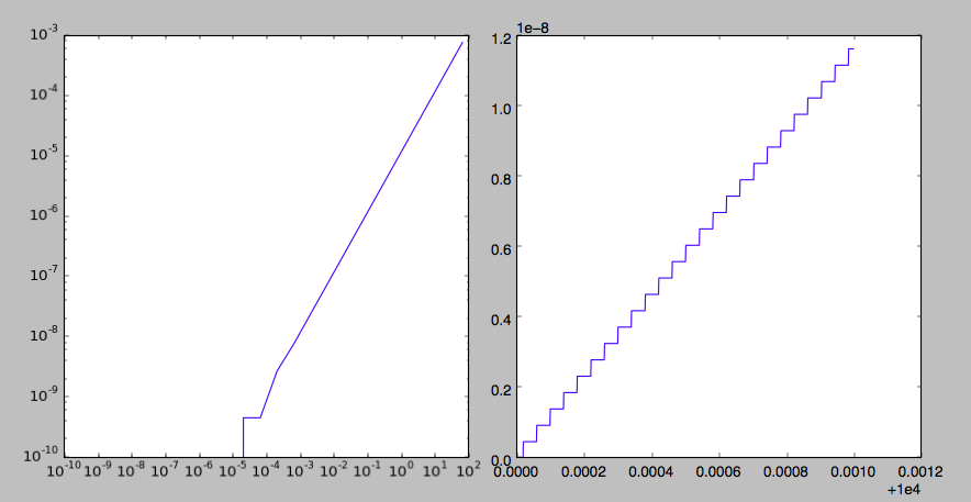
The accepted answer by @pv. explains that Skyfield has a "staircase" response, meaning that some values it returns are locally flat except for discrete jumps.

I did a little experiment on the first step - converting times to JulianDate objects, indeed it looks like roughly 40 microseconds per increment, or about 5E-10 days. That's reasonable, considering the JPL databases span thousands of years. While this is probably fine for almost any general astronomical-scale application, it's not actually smooth. As the answer points out - the local flatness will trigger "success" in some (probably many) minimizers. This is expected and reasonable and is not in any way a failure of the method.

from skyfield.api import load, now, JulianDate
import numpy as np
import matplotlib.pyplot as plt

t  = 10000 + np.logspace(-10, 2, 25)        # logarithmic spacing
jd = JulianDate(utc=(2016, 3, 9, 0, 0, t))

dt  = t[1:] - t[:-1]
djd = jd.tt[1:] - jd.tt[:-1]

t  = 10000 + np.linspace(0, 0.001, 1001)        # linear spacing
jd = JulianDate(utc=(2016, 3, 9, 0, 0, t))

plt.figure()

plt.subplot(1,2,1)

plt.plot(dt, djd)
plt.xscale('log')
plt.yscale('log')

plt.subplot(1,2,2)

plt.plot(t, jd.tt-jd.tt[0])

plt.show()

Goody

Answer 3

I cannot extol too highly the value of the print statement for seeing how an algorithm is behaving through time. If you try adding one to the top of your separation() function, then you will get to see the minimization routines work their way towards an answer:

def separation(seconds, lat, lon):
    print seconds
    ...

Adding this line will let you see that the Nelder-Mead method does a thorough search of the seconds range, striding forward in 500-second increments before it starts to play:

[ 10000.]
[ 10500.]
[ 11000.]
[ 11500.]
[ 12500.]
...

Of course, it does not know these are 500-second increments, because to a solver like these, the problem has no units. These adjustments might be 500 meters, or 500 angstroms, or 500 years. But it stumbles blindly forward and, in the case of Nelder-Mead, sees enough of how the output varies with the input to hone in on an answer you like.

Here, for contrast, is the entire search made by the default algorithm:

[ 10000.]
[ 10000.00000001]
[ 10000.]

That's it. It tries stepping slight away by 1e-8 seconds, cannot see any different in the answer it gets, and gives up — as several of the other answers here correctly asserted.

Sometimes you can fix up a situation like this by telling the algorithm to (a) take a bigger step to start with and (b) stop testing once the step size it is making gets small — say, when it drops to a millisecond. You might try something like:

out_s_def = minimize(separation, sec_init, args=(32.5, 215.1),
                     tol=1e-3, options={'eps': 500})

In this case it still seems that the default minimization technique is too fragile to constructively find the minimum even when given this help, so we can do something else: we can tell the minimization function how many bits it really has to play with.

You see, these minimization routines are often written with a fairly explicit knowledge of how precise a 64-bit float can be pushed before no more precision is available, and they are all designed to stop before that point. But you are hiding the precision: you are telling the routine “give me a number of seconds” which makes them think that they can fiddle with even very tiny low-end digits of the seconds value, when in reality the seconds are getting combined with not just hours and days but with years, and in the process any tiny precision down at the bottom of the seconds is lost — though the minimizer does not know!

So let's expose the real floating-point time to the algorithm. In the process, I'll do three things:

1. Let's avoid the need for the float() maneuver you are doing. Our print statement shows the problem: that even though you provided a scalar float, the minimizer turns it into a NumPy array anyway:

   (array([ 10000.]), 32.5, 215.1)
   

   But that is easy to fix: now that Skyfield has a separation_from() built in that can handle arrays just fine, we will use it:

   sepa = mpos.separation_from(spos)
   return sepa.degrees
   

2. I will switch to the new syntax for creating dates, that Skyfield has adopted as it heads towards 1.0.

That gives us something like (but note that this would be faster if you only built the topos once and passed it in, instead of rebuilding it and making it do its math over every time):

ts = load.timescale()

...

def separation(tt_jd, lat, lon):
    place = earth.topos(lat, lon)
    t = ts.tt(jd=tt_jd)
    mpos = place.at(t).observe(moon).apparent()
    spos = place.at(t).observe(sun).apparent()
    return mpos.separation_from(spos).degrees

...

sec_init = 10000.0
jd_init = ts.utc(2016, 3, 9, 0, 0, sec_init).tt
out_s_def = minimize(separation, jd_init, args=(32.5, 215.1))

The result is a successful minification, giving — I think, if you could double-check me here? — the answer you are looking for:

print ts.tt(jd=out_s_def.x).utc_jpl()

['A.D. 2016-Mar-09 03:37:33.8224 UT']

I hope soon to bundle a number of pre-built minification routines in with Skyfield — in fact, a big reason for writing it to replace PyEphem was wanting to be able to unleash powerful SciPy optimizers and be able to abandon the rather anemic ones that PyEphem implements in C. The main thing they will have to be careful about is what happened here: that an optimizer needs to be given floating point digits to wiggle that are significant all the way down.

Maybe I should look into allowing Time objects to compose their times from two floating point objects, so that many more seconds digits can be represented. I think AstroPy has done this, and it is traditional in astronomy programming.

Embryonic

OK this is great! Indeed I could have used print, but then I never would have learned so much about what is going on "under-the-hood" as I have here by asking for better understanding here in SE. I'm looking forward to 1.0 - these new methods are really worth waiting for. I think it's great to be able to search for criteria like eclipse totality or occultations. Will the time objects ever have a simple add method of their own? – Goody

Oh, I looked back and found that the float() # seems necessary was actually only needed for .topos() which won't work if I accidentally entered latitude or longitude as integers without a decimal. – Goody