Plotting empirical and fitted semivariogram in ggplot

Question

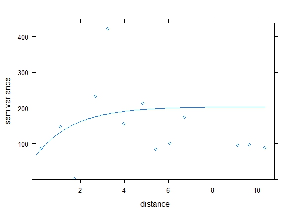
I am investigating spatial autocorrelation in my data using semivariograms. My data:

Response <- c(21L, 36L, 30L, 29L, 30L, 45L, 100L, 0L, 0L, 0L, 0L, 0L, 59L, 
18L, 24L, 23L, 26L, 29L, 23L, 21L, 14L, 30L, 43L, 14L, 8L, 0L, 
0L, 0L, 0L, 0L, 23L, 38L, 20L, 28L, 45L, 21L, 46L, 23L, 6L, 4L, 
0L, 0L, 0L, 0L, 0L, 17L, 10L, 41L, 24L, 31L, 16L, 23L, 31L, 6L, 
2L, 0L, 0L, 0L, 0L, 0L, 8L, 20L, 18L, 18L, 40L, 9L, 1L, 25L, 
4L, 34L, 0L, 0L, 0L, 0L, 0L, 39L, 8L, 7L, 22L, 16L, 18L, 23L, 
11L, 25L, 28L, 0L, 0L, 0L, 0L, 0L, 3L, 22L, 11L, 9L, 123L, 50L, 
12L, 1L, 46L, 1L, 4L, 1L, 2L, 0L, 37L)

Covar1 <- structure(c(1L, 3L, 1L, 1L, 3L, 3L, 1L, 2L, 2L, 2L, 2L, 2L, 1L, 
3L, 3L, 1L, 3L, 1L, 1L, 3L, 3L, 1L, 1L, 3L, 3L, 2L, 2L, 2L, 2L, 
2L, 1L, 3L, 1L, 1L, 3L, 3L, 1L, 1L, 3L, 3L, 2L, 2L, 2L, 2L, 2L, 
1L, 3L, 1L, 1L, 3L, 3L, 1L, 1L, 3L, 3L, 2L, 2L, 2L, 2L, 2L, 1L, 
3L, 1L, 1L, 1L, 3L, 3L, 3L, 3L, 1L, 2L, 2L, 2L, 2L, 2L, 1L, 3L, 
3L, 3L, 3L, 1L, 1L, 3L, 1L, 1L, 2L, 2L, 2L, 2L, 2L, 3L, 3L, 1L, 
3L, 1L, 1L, 3L, 3L, 1L, 2L, 2L, 2L, 2L, 2L, 1L), .Label = c("A", 
"B", "C"), class = "factor")

Covar2 <- structure(c(1L, 1L, 1L, 1L, 1L, 1L, 1L, 1L, 1L, 1L, 1L, 1L, 1L, 
1L, 1L, 2L, 2L, 2L, 2L, 2L, 2L, 2L, 2L, 2L, 2L, 2L, 2L, 2L, 2L, 
2L, 3L, 3L, 3L, 3L, 3L, 3L, 3L, 3L, 3L, 3L, 3L, 3L, 3L, 3L, 3L, 
4L, 4L, 4L, 4L, 4L, 4L, 4L, 4L, 4L, 4L, 4L, 4L, 4L, 4L, 4L, 5L, 
5L, 5L, 5L, 5L, 5L, 5L, 5L, 5L, 5L, 5L, 5L, 5L, 5L, 5L, 6L, 6L, 
6L, 6L, 6L, 6L, 6L, 6L, 6L, 6L, 6L, 6L, 6L, 6L, 6L, 7L, 7L, 7L, 
7L, 7L, 7L, 7L, 7L, 7L, 7L, 7L, 7L, 7L, 7L, 7L), .Label = c("1", 
"2", "3", "4", "5", "6", "7"), class = "factor")

df <- data.frame(Response, Covar1, Covar2)

I run a simple model, use gstat to make both empirical and fitted semivariograms from the residuals and spatial coordinates, and plot them:

mod1 <- glm(Response ~ Covar1 * Covar2, data = df)

geo <- as.data.frame(resid(mod1))

geo$x <- c(34.59481, 34.60548, 34.59825, 34.59039, 34.56546, 34.56749, 
34.5964, 34.40986, 34.40083, 34.39536, 34.41291, 34.40512, 34.36381, 
34.35335102, 34.32548, 34.59481, 34.60548, 34.59825, 34.59039, 
34.56749, 34.56546, 34.5964, 34.36381, 34.35335102, 34.32548, 
34.41291, 34.40986, 34.40512, 34.40083, 34.39536, 34.59481, 34.60548, 
34.59825, 34.59039, 34.56749, 34.56546, 34.5964, 34.36381, 34.35335102, 
34.32548, 34.41291, 34.40986, 34.40512, 34.40083, 34.39536, 34.59481, 
34.60548, 34.59825, 34.59039, 34.56749, 34.56546, 34.5964, 34.36381, 
34.35335102, 34.32548, 34.41291, 34.40986, 34.40512, 34.40083, 
34.39536, 34.59481, 34.60548, 34.59825, 34.59039, 34.36381, 34.35335102, 
34.32548, 34.56749, 34.56546, 34.5964, 34.41291, 34.40986, 34.40512, 
34.40083, 34.39536, 34.36381, 34.35335102, 34.32548, 34.56546, 
34.56749, 34.5964, 34.59481, 34.60548, 34.59825, 34.59039, 34.41291, 
34.40986, 34.40512, 34.40083, 34.39536, 34.32548, 34.35335102, 
34.59481, 34.60548, 34.59039, 34.59825, 34.56546, 34.56749, 34.5964, 
34.41291, 34.40986, 34.40512, 34.40083, 34.39536, 34.36381)

geo$y <- c(-2.18762, -2.18308, -2.16174, -2.16018, -2.14787, -2.15296, 
-2.12863, -2.14325, -2.14552, -2.1454, -2.13926, -2.14652, -2.12463, 
-2.121925978, -2.10213, -2.18762, -2.18308, -2.16174, -2.16018, 
-2.15296, -2.14787, -2.12863, -2.12463, -2.121925978, -2.10213, 
-2.13926, -2.14325, -2.14652, -2.14552, -2.1454, -2.18762, -2.18308, 
-2.16174, -2.16018, -2.15296, -2.14787, -2.12863, -2.12463, -2.121925978, 
-2.10213, -2.13926, -2.14325, -2.14652, -2.14552, -2.1454, -2.18762, 
-2.18308, -2.16174, -2.16018, -2.15296, -2.14787, -2.12863, -2.12463, 
-2.121925978, -2.10213, -2.13926, -2.14325, -2.14652, -2.14552, 
-2.1454, -2.18762, -2.18308, -2.16174, -2.16018, -2.12463, -2.121925978, 
-2.10213, -2.15296, -2.14787, -2.12863, -2.13926, -2.14325, -2.14652, 
-2.14552, -2.1454, -2.12463, -2.121925978, -2.10213, -2.14787, 
-2.15296, -2.12863, -2.18762, -2.18308, -2.16174, -2.16018, -2.13926, 
-2.14325, -2.14652, -2.14552, -2.1454, -2.10213, -2.121925978, 
-2.18762, -2.18308, -2.16018, -2.16174, -2.14787, -2.15296, -2.12863, 
-2.13926, -2.14325, -2.14652, -2.14552, -2.1454, -2.12463)

library(sp)     
names(geo) <- c("resids", "x", "y")
coordinates(geo) <- ~ x + y
proj4string(geo) <- CRS("+proj=longlat +datum=WGS84")

library(gstat)
var1 <- variogram(resids ~ x + y, data = geo)
v.fit1 = fit.variogram(var1, vgm(50, "Exp", 2, 50))
plot(var1, v.fit1)

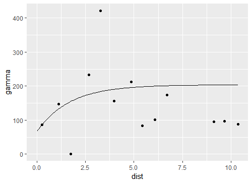
The plot is class 'trellis', which doesn't take arguments from standard base R graphics, so I would instead like to use ggplot to create my figure. I can plot my empirical variogram (the points only):

ggplot(var1, aes(x=dist,y=gamma)) +
geom_point()

But I'm having trouble plotting the fitted model (the line). Any help would be much appreciated.

Leavening

can you try geom_smooth(method = "glm") or "lm", "gam", "loess", "rlm" – Rena

Answer 1

You can generate semivariance values for a given variogram model via variogramLine() from package gstat. You can then use those in geom_line() to draw those fitted values.

I only get values out to the max distance in var1 so the range of the two datasets will be the same.

preds = variogramLine(v.fit1, maxdist = max(var1$dist))
head(preds)
          dist    gamma
1 1.037174e-05 67.13427
2 5.212964e-02 71.24628
3 1.042489e-01 75.23463
4 1.563682e-01 79.10305
5 2.084874e-01 82.85514
6 2.606067e-01 86.49440

Now add a geom_line() layer to the plot, using this new dataset. The names of the x and y variables are the same as in var1 so you don't need to map any new aesthetics.

ggplot(var1, aes(x = dist, y = gamma)) +
     geom_point() +
     geom_line(data = preds)

Damaging

Answer 2

Just adding something useful after the very insightful answer from aosmith. You might want to add proportional points in your empiric variogram. I managed to do so using the following code:

plot_variogram <- function(v, m) {
  preds = variogramLine(m, maxdist = max(v$dist))
  ggplot() + 
    geom_point(data = v, aes(x = dist, y = gamma, size=np)) +
    geom_line(data = preds, aes(x = dist, y = gamma))
}

v <- variogram(zinc ~ 1, meuse)
m <- fit.variogram(v, vgm(c("Exp", "Sph")))
plot_variogram(v, m) 

You can check this post for more theming: Variography with gstat and ggplot2

Greenfield