I'm trying to create a map in R that conveys both the shape of underlying geometry (i.e., the physical boundaries) and the relative importance of the object in terms of an associated value.

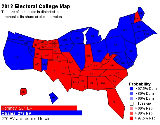
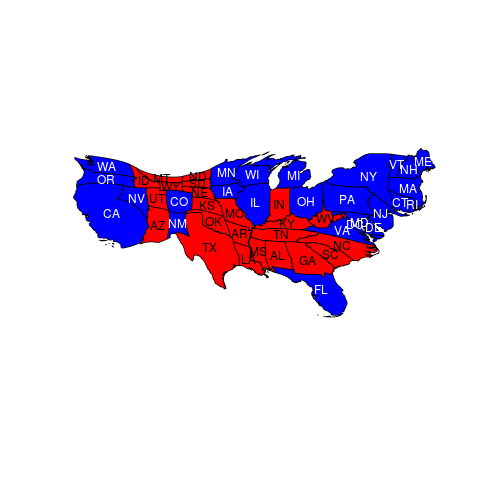
For concreteness, I'd like to focus on reproducing (a version of) the following map* (the shapes, not so much the colors since I can't find the polling data):

I also don't want to bother with getting Alaska and Hawaii to appear below the US instead of in their geodesically correct locations.

I'm only as far as getting the data merged with the weights, done for example as follows:

1. Get polygons

library(maptools)
library(data.table) #not strictly necessary but I prefer it
#US states downloaded (500k resolution) from:
#https://www.census.gov/geo/maps-data/data/cbf/cbf_state.html
us.states<-
  readShapePoly("~/Desktop/cb_2014_us_state_5m.shp")

setDT(us.states@data)

#for getting rid of territories, AK, HI
states<-sprintf("%02d",1:59)
ak.hi<-c("02","15")

us.states.contig<-
  us.states[us.states@data$STATEFP %in% 
              setdiff(states,ak.hi),]

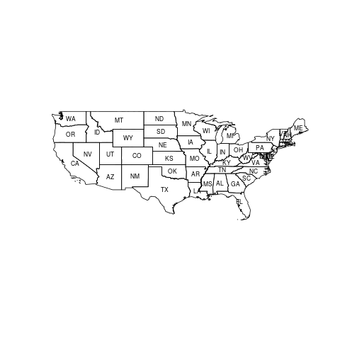
#Unadorned plot
plot(us.states.contig)
text(coordinates(us.states.contig),
     us.states.contig@data[,paste0(STUSPS)],
     cex=.7)

2. Add Electoral College data

#scraped from government page
library(rvest) #only necessary to scrape table
electoral.college.url<-
  paste0("http://www.archives.gov/federal-register/",
         "electoral-college/allocation.html")

electoral.college.dt<-
  (html(electoral.college.url) %>%
     html_nodes("table"))[[5]] %>% 
  html_table()
setDT(electoral.college.dt)
setnames(electoral.college.dt,c("State","Votes"))

#merge into geodata
us.states.contig@data<-
  copy(us.states.contig@data)[
    electoral.college.dt,electoral.votes:=i.Votes,
    on=c(NAME="State")]

#plot, coloring each state by size
states.ranked<-
  us.states.contig@data[,rank(electoral.votes,
                              ties.method="first")]
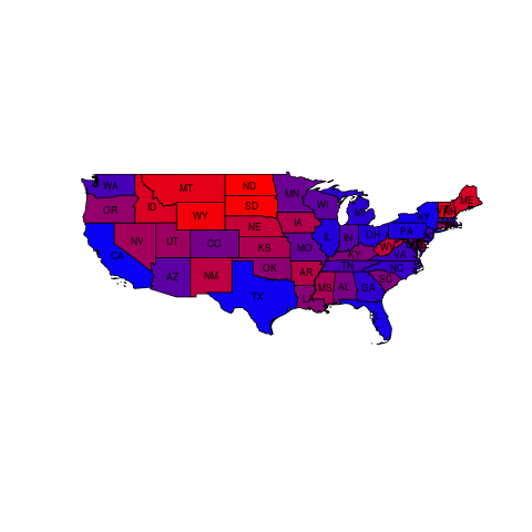
cols<-colorRampPalette(c("red","blue"))(51)[states.ranked]

plot(us.states.contig,col=cols)

This is all well and good--with a glance at this map, we can tell which states have high & low representation in the electoral college. But what if (as in our target map) we wanted to represent another variable with the color of the state?

3. Add 2012 Elections outcomes

#scrape again
#2012 Election Results by State
election.wiki<-
  paste0("https://en.wikipedia.org/wiki/",
         "United_States_presidential_election,_2012")
         
results<-
  html(election.wiki) %>%
  html_node(xpath='//*[@id="mw-content-text"]/div[22]/table') %>%
  html_table()
#eliminate second header row, delete final row,
#  keep only the important columns
results.trim<-results[2:(nrow(results)-1),c(1,4,21)]
colnames(results.trim)<-c("name","pct","abbr")
results.dt<-setDT(results.trim)
#data idiosyncrasies, see Wiki page
results.dt<-results.dt[!grepl("–",abbr)|grepl("a",abbr)]
results.dt[grepl("–",abbr),abbr:=gsub("–.*","",abbr)]
results.dt[,"pct":=as.numeric(gsub("%","",pct))]

#merge
us.states.contig@data<-
  copy(us.states.contig@data
       )[results.dt,vote.pct:=i.pct,
         on=c(STUSPS="abbr")]
                              
pcts<-us.states.contig@data[,vote.pct]
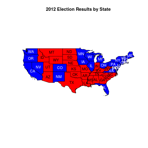
cols<-c("red","blue")[(pcts>=50)+1L]
tx.col<-c("white","black")[(cols=="red")+1L]
plot(us.states.contig,col=cols)
text(coordinates(us.states.contig),
     us.states.contig@data[,paste0(STUSPS)],
     col=tx.col)

This last graph gets at the crux of the issue. The first graph presented is far superior in the sense that we can sense from the percentage red vs. blue of the map whether the Republicans or Democrats won; this last map is misleading because the most Republican states are also the most sparsely-populated.

Is there any way to create a distorted version of this map which conveys the relative importance of each state in the electoral college? I couldn't find any help online, perhaps mainly because I don't know if there's a standard name for this type of graph.

*This map was found here; I've seen similar size-distorted maps before, e.g. in The Economist. It appears it's based on the work of Dr. Sam Wang at Princeton's Election Consortium and was produced by Drew Thaler.

Following the advice of package maintainer @chkaiser, I've sought out and finally discovered a way to do this within R. This blog post was a tremendous help and the getcartr package is fantastic.

First, get the Rcartogram and getcartr packages from GitHub:

remotes::install_github("omegahat/Rcartogram")
remotes::install_github('chrisbrunsdon/getcartr', subdir='getcartr')
library(Rcartogram)
library(getcartr)

Now simply plug & chug:

us.states.contig.carto = quick.carto(
  us.states.contig,
  us.states.contig@data$electoral.votes
)
plot(us.states.contig.carto, col = cols)
text(
  coordinates(us.states.contig.carto),
  us.states.contig@data[ , paste0(STUSPS)],
  col = tx.col
)

And just like that we have our cartogram:

1. Get polygons

2. Add Electoral College data

3. Add 2012 Elections outcomes

Recommended topics

Hot tags