Combining choropleth made in ggplot and ggmap

Question

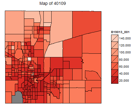
Created a choropleth using ggplot2. Here's the ggplot code

okc <- ggplot() +
  geom_polygon(data = mapdata, aes(x = long, y = lat, group = group,
                                   fill = B19013_001), color = "black", size = 0.5)+
  scale_fill_distiller(palette = "Reds", labels = comma,
                       breaks = pretty_breaks(n = 10), values = c(1,0)) +
  guides(fill = guide_legend(reverse = TRUE)) +
  theme_nothing(legend = TRUE) +
  ggtitle('Map of 40109') 

Here's a sample of the data from mapdata:

       long      lat order  hole piece         group          id
1 -97.54285 35.51951     1 FALSE     1 40109100100.1 40109100100
2 -97.54282 35.51954     2 FALSE     1 40109100100.1 40109100100
3 -97.54280 35.51963     3 FALSE     1 40109100100.1 40109100100
4 -97.54276 35.51976     4 FALSE     1 40109100100.1 40109100100
5 -97.54270 35.51993     5 FALSE     1 40109100100.1 40109100100
6 -97.54266 35.52016     6 FALSE     1 40109100100.1 40109100100
                                          NAME state county  tract B19013_001
1 Census Tract 1001, Oklahoma County, Oklahoma    40    109 100100      33440
2 Census Tract 1001, Oklahoma County, Oklahoma    40    109 100100      33440
3 Census Tract 1001, Oklahoma County, Oklahoma    40    109 100100      33440
4 Census Tract 1001, Oklahoma County, Oklahoma    40    109 100100      33440
5 Census Tract 1001, Oklahoma County, Oklahoma    40    109 100100      33440
6 Census Tract 1001, Oklahoma County, Oklahoma    40    109 100100      33440

It produced this plot.

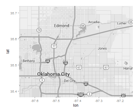
I also created a roadway map using ggmap. Here's the code:

map <- get_map(location = c(lon = mean(mapdata$lon), lat = mean(mapdata$lat))
               , zoom = 10
               , maptype = "roadmap"
               , color = "bw")
p <- ggmap(map) +
  scale_x_continuous(limits = c(min(mapdata$lon), max(mapdata$lon)), expand = c(0, 0)) +
  scale_y_continuous(limits = c(min(mapdata$lat), max(mapdata$lat)), expand = c(0, 0))
p

And here's the map it produces.

When I try to combine them though I get an error. Here's the code I use to combine them and the error:

okc <- okc + p

Error in p + o : non-numeric argument to binary operator
In addition: Warning message:
Incompatible methods ("+.gg", "Ops.data.frame") for "+"

I'm not sure why I'm getting this error. Is it because the maps are not scaled the same? I could not figure how else to scale ggmap other than using the very imprecise zoom function. If anyone has any ideas about how to layer the choropleth on top of the ggmap I will be very thankful.

Here's the rest of the code to recreate the ggplot choropleth.

    library(acs)
    library(ggplot2)
    library(ggmap)
    library(UScensus2010)
    library(RColorBrewer)
    library(dplyr)
    library(scales)

    #http://api.census.gov/data/key_signup.html
    api.key.install(key="c369cd6ed053a84332caa62301eb8afe98bed825")

    # Load in Shape File (You'll need to download this file from the census)
    #ftp://ftp2.census.gov/geo/tiger/TIGER2013/TRACT/tl_2013_40_tract.zip

    ## load, subset shapefile
    geodat<-readShapePoly("insert shapefile here", proj4string=CRS('+proj=longlat +datum=NAD83'))
    geodat<-geodat[geodat$COUNTYFP==109,]

    ## fortify for ggplot digestion
    geodat.f<-fortify(geodat,region="GEOID")

    # American Community Survey Data: Median HH Income for OK Census Tracts
    ok.counties=geo.make(state="OK", county="Oklahoma", tract="*")
    ok.income<-acs.fetch(geography=ok.counties, table.number="B19013", endyear=2013)


    # Merge Data Sets 
    geo_dat<-geography(ok.income)
    var_dat<-as.data.frame(estimate(ok.income))
    acs_data<-cbind(geo_dat,var_dat)
    acs_data$id<- paste("40109", acs_data$tract, sep = "")

    ## from dplyr
    mapdata<-left_join(geodat.f,acs_data)

    okc <- ggplot() +
      geom_polygon(data = mapdata, aes(x = long, y = lat, group = group,
                                       fill = B19013_001), color = "black", size = 0.5)+
      scale_fill_distiller(palette = "Reds", labels = comma,
                           breaks = pretty_breaks(n = 10), values = c(1,0)) +
      guides(fill = guide_legend(reverse = TRUE)) +
      theme_nothing(legend = TRUE) +
      ggtitle('Map of OKC')

Introspect

With the provided data, I cannot really do a lot. Since you want to draw polygons on top of a map, you want to do something like this: ggmap(map) + geom_polygon(data = mapdata, aes(x = long, y = lat, group = group, fill = B19013_001), color = "black", size = 0.5) I think you want to provide a base layer, which is a map, using ggmap() then you draw polygons on top of it. – Preside

@Preside Yeah, that's exactly what I'm trying to do. The code you provided is a good start but it stacks the choropleth on top of the roadway map. Is there a way to change the opacity of the choropleth so that you can actually see what is underneath? – Introspect

I see. In that case, you want to use alpha in geom_polygon(). You can do; ggmap(map) + geom_polygon(data = mapdata, aes(x = long, y = lat, group = group, fill = B19013_001), color = "black", size = 0.5, alpha = 0.5). Play with the alpha value (between 0 and 1) and see which value gives you the right image. – Preside

By the way, you may want to provide the shape file you use. Just saying "insert shapefile here" would not allow SO users to help you out. – Preside

@Preside how can I directly add it? I inserted a link to the shapefile above but wouldn't someone trying to run the code have to download it and save it to their own system? – Introspect

If all materials are there, I will try to have a look and help you. If you already found your way, you don't have to. :) – Preside

Answer 1

This is actually much better done in Leaflet. It looks better aesthetically and also code wise it is more intuitive.

library(leaflet)
library(rgdal)
library(RColorBrewer)

pal <- colorNumeric("OrRd", domain = new$pct_minority_popn)

leaflet(mapdata) %>%
 addTiles %>%
 addPolygons(stroke=T, fillOpacity=.5, smoothFactor=.5, color=~pal(B19013_001)) %>%
 addLegend("bottomright", pal=pal, values=~B19013_001, title="Legend Title", opacity=.8)

You can change the bottom map by replacing the addTiles command with something like addProviderTiles("CartoDB.Positron"). You can see the rest of the options and more info on leaflet at: https://rstudio.github.io/leaflet/basemaps.html

Tallulah