Calculate Impulse/Torque for both bodies in a 3D fix joint constraint

Question

I have 2 rigid bodies (a & b) and 1 fix joint constraint (with relative transformation rela).

My objectives are to achieve :-

No. 1. b.transform = a.transform * rela
No. 2. Center of mass (a+b) doesn't change.
No. 3. (3rd Newton rule) Velocity of total system (a+b) doesn't change.
No. 4. (3rd Newton rule) Angular velocity of total system (a+b) doesn't change.
No. 5. Moving/rotating of both objects to solve it should be minimized.

I wish to apply impulse/torque to both bodies to make them gradually meets the requirement.
This video can depict what I want - (youtube link).

How to solve the value of impulse/torque that apply for each body?
I want a rough idea / algorithm.
It can be a description text without any code.

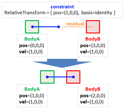
Example

Here is a sample problem and its correct solution (i.e. final resting state) :-

Code (draft)

Here is my current snippet, just in case :-

class Transform {
    Vec3 pos;
    Matrix33 basis;
};

Each rigid body has these fields :-

class RigidBody {
    float mass;
    Matrix33 inertiaTensor;
    Transform transform;
    Vec3 velocity;
    Vec3 angularVelocity;
};

The fix joint constraint is :-

class FixConstraint {
    Transform rela;
    RigidBody* a;
    RigidBody* b;
};

Draft of my poor solution

In nutshell, I have to modify 12 variables.

• position of a and b (xyz - 6 variables)
• orientation of a and b (angle xyz - 6 variables)

Then I can use "My objectives" No 1 & 2 to create some equations.
Then, at best, I have to solve 12 linear equation with 12 unknown variables.
I doubt if it has to be that hard.

My previous internet search

I have looked into various sources, but they mostly :-

• just drive into iteration solver.
• try to diagonalize matrix + jacobian : only expert can understand.
• "Why don't you look into (insert name of Physic Engine here) source code?" without beginner-friendly explanation.
• show how to use (name of Physic Engine) to create a fix joint constraint.

Here are some of the most useful ones :-

• Bullet Physics solver : https://github.com/svn2github/bullet/blob/master/tags/bullet-1.5f/BulletDynamics/ConstraintSolver/Point2PointConstraint.cpp
• "Stable, Robust, and Versatile Multibody Dynamics Animation" research paper http://image.diku.dk/kenny/download/erleben.05.thesis.pdf (see chapter 6)
• (edited-add) Featherstone's algorithm for ragdoll : https://en.wikipedia.org/wiki/Featherstone%27s_algorithm (but it focuses on many constraints rather than one)

(edited some wording and rule, thank fafl and Nico Schertler.)

---

(edited-add, after a few days)
I believe if I can crack "Point2PointConstraint.cpp" (of the Bullet Physics), I will be fully understand the algorithm and principle.

I also copy-paste it here, just in case.
Here is the first part :-

SimdVector3 normal(0,0,0);
for (int i=0;i<3;i++)
{
    normal[i] = 1;
    new (&m_jac[i]) JacobianEntry(
        m_rbA.getCenterOfMassTransform().getBasis().transpose(),
        m_rbB.getCenterOfMassTransform().getBasis().transpose(),
        m_rbA.getCenterOfMassTransform()*m_pivotInA - m_rbA.getCenterOfMassPosition(),
        m_rbB.getCenterOfMassTransform()*m_pivotInB - m_rbB.getCenterOfMassPosition(),
        normal,
        m_rbA.getInvInertiaDiagLocal(),
        m_rbA.getInvMass(),
        m_rbB.getInvInertiaDiagLocal(),
        m_rbB.getInvMass());
    normal[i] = 0;
}

Here is the second part :-

SimdVector3 pivotAInW = m_rbA.getCenterOfMassTransform()*m_pivotInA;
SimdVector3 pivotBInW = m_rbB.getCenterOfMassTransform()*m_pivotInB;
SimdVector3 normal(0,0,0);
for (int i=0;i<3;i++)
{       
    normal[i] = 1;
    SimdScalar jacDiagABInv = 1.f / m_jac[i].getDiagonal();

    SimdVector3 rel_pos1 = pivotAInW - m_rbA.getCenterOfMassPosition(); 
    SimdVector3 rel_pos2 = pivotBInW - m_rbB.getCenterOfMassPosition();
    //this jacobian entry could be re-used for all iterations

    SimdVector3 vel1 = m_rbA.getVelocityInLocalPoint(rel_pos1);
    SimdVector3 vel2 = m_rbB.getVelocityInLocalPoint(rel_pos2);
    SimdVector3 vel = vel1 - vel2;

    SimdScalar rel_vel;
    rel_vel = normal.dot(vel);

    //positional error (zeroth order error)
    SimdScalar depth = -(pivotAInW - pivotBInW).dot(normal); //this is the error projected on the normal

    SimdScalar impulse = depth*m_setting.m_tau/timeStep  * jacDiagABInv -  m_setting.m_damping * rel_vel * jacDiagABInv;

    SimdVector3 impulse_vector = normal * impulse;
    m_rbA.applyImpulse(impulse_vector, pivotAInW - m_rbA.getCenterOfMassPosition());
    m_rbB.applyImpulse(-impulse_vector, pivotBInW - m_rbB.getCenterOfMassPosition());

    normal[i] = 0;
}

Fabulist

Just to clarify, you have two moving and rotating bodies and want to set their distance from each other to a constant? If they are further apart, do you "teleport" them closer? Should the resulting body spin? Will each of the bodies spin after the fixing (like wheels on a car) or do they spin as one (like wheels on a car but with brakes engaged)? – Hageman

@Hageman Yes, constant, or at least near-constant (it is soft-constraint). Actually, I would love to see they move close together using impulse and torque, with correct Newton's third law about action/reaction (between a and b). However, it is quite hard, so teleporting is not too bad. About the spinning : If a is on the left and moving up, and b is one the right and moving down, if they may join together, the overall result should roughly spin-as-one in clockwise direction. (I edited question a little, thanks.) – Fabulist

In the moment of joining, will the bodies stop spinning individually? Is the connection always placed in the center of each body? – Hageman

@Hageman 1. Yes, it should gradually stop spinning individually. How gradual, it depends on strength of constraint. (But if it is too hard, it is ok to stop spinning individually abruptly.) 2. No. – Fabulist

@Hageman This link can depict what I want : youtube.com/watch?v=b4k2Q0i39fY&feature=youtu.be&t=23 . Notice that the constraint is sometimes violated a little bit. XD – Fabulist

Here are some of my thoughts before any further analysis (note that I am not a physicist): The rotation of both objects should not have an impact on the angular or linear velocity of the total system. Therefore, you can treat both objects as mass points and only need to solve for the translations to apply to both objects. Rule 2 implies that both translations are coupled and somewhat complementary. Hence, if you know one, you know the other. Rule 2 should automatically imply rule 3. Rule 4 is another constraint on the velocity and probably implies that it points towards the common centroid... – Cryptozoite

The only thing left to solve for is the magnitude of a single translation, which you can just define by proposing a weight of the constraint. All other unknowns should follow from there. – Cryptozoite

@Nico Schertler That is useful. I will try to solidify it. Thanks. – Fabulist

@Fabulist I would handle the 2 objects as single one. so single center of mass, apply all forces to this center of mass... that should handle the overal relative rotation of bodies and movement. And also apply the same forces to the bodies it self but ignore them for movement use them just for local rotations. If such rotation create another force impulse (either due to friction or non spherical surface) apply it to the center of mass of the a+b object instead. – Pecksniffian

@Pecksniffian 1. How? If I apply force to CM, how that would handle the overall relative transformation? 2. I don't care about collision response/detection (and any friction). 3. I feel good about your comment (like dividing the problem), but I can't grasp it. 4. Thank! – Fabulist

@Fabulist You know what reper (moving trilateral) is? Basically its a 4x4 transform matrix describing a 3D coordinate system of your a+b object. Origin is the center of mass of the objects combined and axises are aligned so the objects are in single line/axis (for example x) in each update apply rotations and movement to this reper and compute global position of the sub objects from it ... as their local coordinates would be always the same ... so its just matter of multiplying by direct or inverse matrix (depending on the notations used) – Pecksniffian

@Fabulist frictions are important otherwise a rotating ball would not move on the plane ... btw the reper is similar toTBN matrix (tangen, bi-normal, normal) but TBN is missing position ... – Pecksniffian

@Pecksniffian I use 4x4 and TBN in Opengl, but never heard of reper/trilateral. Thank for explanation. :) I frequently use this formula absoluteTransformChild = absoluteTransformParent*relativeTransformOfThatChild. (just in case if it is what you are explaining) ; Hmm, I still don't believe friction is related to this question. I agree that friction makes rotating ball move on a floor. – Fabulist

@Fabulist if your balls are not rotating (around own local axises) then you do not need friction indeed ... yes the 4x4 transform matrices from OpenGL are the same as reper ... you can use them for physics computation too ... its also common in robotics for direct and inverse kinematics representation in algebraic form but that is a different topic.... – Pecksniffian

Answer 1

As the name suggests, a constraint is a restriction imposed on the movement of two bodies. Hence to successfully model a constraint, one must fully understand what restrictions that constraint imposes on the two bodies and represent those constraints as an impulse or force equation. Impulse-based solvers are used over force-based solvers almost all the time since first-order (velocity) equations (and the numbers involved) are easier to compute and deal with than second-order (acceleration) equations. We will thus be looking at modelling impulses for general 1-D constraints (n-D constraints can be represented as one or more 1-D constraints).

Modelling the first-order (velocity) restriction of a 1-D constraint

The first step in modelling a constraint with impulses is representing the restriction(s) as first-order (velocity/momentum) equations. The fixed constraint in question (henceforth simply referred to as "the constraint") has a simple positional (zeroth order) restriction: the linear and angular positions in constraint space must stay the same (as specified by the relative transform rela). We can convert this into a first order restriction by levying the fact that in order to make the relative position of two bodies constant, their relative velocity must be zero. The constraint can thus be interpreted as ensuring that the relative linear and angular velocities of the two bodies in constraint space are zero.

The constraint can now be modeled as an impulse which must be applied to the system so that the relative velocity becomes zero. If v1 and v2 are the initial and final relative velocities of the system, m is the mass of the system and j is the impulse applied to satisfy the constraint, then

v2 = v1 + j/m    (1)
v2 = 0           (2)

The first equation holds true for any constraint (it is Newton's second law), but the second equation (henceforth referred to as the constraint equation) only holds true for the given constraint.

Modelling the zeroth-order (position) restriction of a 1-D constraint

Our model now ensures that the relative position stays constant (first-order restriction), but we still haven't enforced the zeroth-order restriction, i.e. the relative position of B with respect to A must be that which is specified by the relative transform rela. If x1 is the "error" in the constraint system position, then this can be "injected" into the impulse using a Baumgarte term beta * x1/h where h is the time step and beta is a parameter typically between 0 and 1. You can consider beta to be the fraction of the positional error you want the solver to resolve every frame.

Our constraint equation now becomes

v2 + beta*x1/h = 0

Note: If the solver uses semi-implicit integration, then x1 is the initial positional error, but if the solver uses implicit integration the error is actually x2 = x1 + v2*h.

Damping/softening the constraint

As you pointed out, the constraint you are looking for is a soft (or damped) constraint, since you want the movement to happen gradually. To damp the constraint exponentially, we simulate the exponential decay differential equation and add a value proportional to j (which is proportional to derivative of velocity dv = v2 - v1 as the time step gets infinitesimally small).

Our constraint equation now becomes

v2 + beta * x1/h + gamma * j = 0

Where gamma >= 0 is another parameter (also called the damping coefficient). If gamma = 0, the constraint will be undamped or rigid.

Eliminating v2 from the two equations and solving the resulting equation for j gives us

j = -(v1 + beta * x1/h) * (1/(gamma + 1/m))
                         | equivalent mass |

The solver applies this impulse and its negative in the direction of the axis (typically called the normal) of the constraint.

Adapting and using the general 1-D soft constraint

This general 1-D soft constraint impulse can be repurposed to create many different joints, like fixed joints, spring joints and so on. For a fixed joint, we want the constraint to constrict B's position and rotation in A's space to be the position and rotation of the relative transform. Thus, in A's space, x1 = B.position - rela.origin and v1 = relative velocity of A and B along x1. However, since we want to restrict the position in 3 dimensions (i.e. x1 is a 3d vector, not a scalar), we can solve the 1-D constraint on each of the three axes individually. This process can then be repeated for angular positions and velocities using the same constraint. The same process can be followed to derive the impulse for for any 1-D constraint.

Applying the constraint

Once computed, the impulse j must be applied to both the bodies in opposite directions so that the total impulse on the constraint system is zero. When positive, this impulse is meant to push the two bodies away, and when negative it means to pull them together. Hence, if the constraint normal points from body A to body B (as per convention), -j * normal is applied on body A and +j * normal is applied on body B.

The 1-D constraint can be extended to n-D if needed. Some constraints like the spring/distance constraint are along a line and hence are 1-D constraints by nature in n dimensional space and do not require multiple solution iterations for different axes.

You can also modify the constraint equation to take into account accumulated impulses while damping for stability if your solver uses warm starts. The damping term becomes gamma * (j + j0), where j0 is the accumulated impulse which is applied during the warm start.

Differences with Bullet 1.5 constraint solvers

It must be pointed out that the fixed constraint that you're looking for is actually Generic6DofConstraint (with all 6 degrees of freedom restricted) and not Point2PointConstraint (which is a ball and socket-like joint) in Bullet 1.5. You can look at its implementation for reference. The Bullet 1.5 constraint solvers use a slightly different (and slightly more hand-wavy) damped impulse equation (where they multiply the relative velocity with the damping factor but do not add it to the reciprocal of the equivalent mass) which damps the constraint a bit more. It's up to preference which one you want to choose, but I consider the one used here more justifiable and also much easier to adapt to other naturally soft constraints (for instance, parameterizing the constraint in terms of the spring frequency and damping ratio to simulate a damped spring).

You can also take a look at the hopefully self-explanatory code of the damped spring (soft distance constraint) solver in my 2D physics engine.

Branscum

Ops, agree ... I was wrong at the Point2PointConstraint. Thank +1. I will read the rest of the answer later. XD – Fabulist

No worries, it is a lot to take in :) – Branscum

Cleaned the answer up a little bit and added a section regarding the application of the impulse on the bodies. I will add a section on the "constraint mass" (also referred to as the Jacobian) and its significance soon. – Branscum

I incorrectly referred to the constraint mass as the Jacobian in the comment above -- the Jacobian is a vector of the coefficients of the linear and angular velocities in the differentiated first-order constraint. – Branscum

Everything is clear until I reached the phrase can be "injected" into the impulse using a Baumgarte term. I guess the term is some kind of bias, but I can't find any good Math formula/principle to back it up. (I am a type that love proving before believing.) The closest link I found is Baumgarte's wiki biography. – Fabulist

By the way, I noticed experts saying a lot about semi-implicit / implicit, especially box2d.org/files/GDC2011/GDC2011_Catto_Erin_Soft_Constraints.pdf (page 15-16) and en.wikipedia.org/wiki/Semi-implicit_Euler_method (more of a reference than a teaching material). I will try to read them again after you explain the Baumgarte-injection. XD – Fabulist

You can think of Baumgarte positional correction as applying velocity to correct the error in the next frame. If the positional error is to be corrected in the next frame, the velocity to be applied is x1 / h. We fix a fraction of this error rather than all of it every frame to prevent jitter and to let the system reach a natural equilibrium easily. The beta parameter is a result of experimentation and is set to a value (usually between 0.05-0.2) after testing. Note that the error is positive when the bodies are to be pulled together, and negative when the bodies are to be pushed away. – Branscum