Bootstrapping a vector of results, by group in R
Asked Answered
J

2

7

Question: How can I use a boostrap to get confidence intervals for a collection of statistics calculated on the eigenvalues of covariance matrices, separately for each group (factor level) in a data frame?

Problem: I can't quite work out the data structure I need to contain these results suitable for the boot function, or a way to "map" the bootstrap over groups and obtain confidence intervals in a form suitable for plotting.

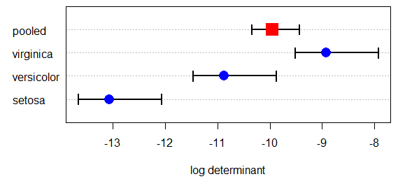
Context: In the heplots package, boxM calculates Box's M test of equality of covariance matrices. There is a plot method that produces a useful plot of the log determinants that go into this test. The confidence intervals in this plot are based on an asymptotic theory approximation.

> library(heplots)
> iris.boxm <- boxM(iris[, 1:4], iris[, "Species"])
> iris.boxm

        Box's M-test for Homogeneity of Covariance Matrices

data:  iris[, 1:4]
Chi-Sq (approx.) = 140.94, df = 20, p-value < 2.2e-16

> plot(iris.boxm, gplabel="Species")

plot of log determinants for Iris data

The plot method can also display other functions of the eigenvalues, but no theoretical confidence intervals are available in this case.

op <- par(mfrow=c(2,2), mar=c(5,4,1,1))
plot(iris.boxm, gplabel="Species", which="product")
plot(iris.boxm, gplabel="Species", which="sum")
plot(iris.boxm, gplabel="Species", which="precision")
plot(iris.boxm, gplabel="Species", which="max")
par(op)

enter image description here

Thus, I would like to be able to calculate these CIs using a boostrap, and display them in the corresponding plots.

What I've tried:

Below are functions that boostrap these statistics, but for the total sample, not taking group (Species) into account.

cov_stat_fun <- function(data, indices, 
            stats=c("logdet", "prod", "sum", "precision", "max")
            ) {
    dat <- data[indices,]
    cov <- cov(dat, use="complete.obs")
    eigs <- eigen(cov)$values

    res <- c(
        "logdet" = log(det(cov)),
        "prod" = prod(eigs),
        "sum" = sum(eigs),
        "precision" = 1/ sum(1/eigs),
        "max" = max(eigs)
        )
}

boot_cov_stat <- function(data, R=500,  ...) {
    boot(data, cov_stat_fun, R=R,  ...)
}

This works, but I need the results by group (and also for the total sample)

> iris.boot <- boot_cov_stat(iris[,1:4])
>
> iris.ci <- boot.ci(iris.boot)
> iris.ci
BOOTSTRAP CONFIDENCE INTERVAL CALCULATIONS
Based on 500 bootstrap replicates

CALL : 
boot.ci(boot.out = iris.boot)

Intervals : 
Level      Normal              Basic             Studentized     
95%   (-6.622, -5.702 )   (-6.593, -5.653 )   (-6.542, -5.438 )  

Level     Percentile            BCa          
95%   (-6.865, -5.926 )   (-6.613, -5.678 )  
Calculations and Intervals on Original Scale
Some BCa intervals may be unstable
>

I also have written a function that calculates the separate covariance matrices for each group, but I can't see how to use this in my bootstrap functions. Can someone help?

# calculate covariance matrices by group and pooled
covs <- function(Y, group) {
   Y <- as.matrix(Y)
   gname <- deparse(substitute(group))
   if (!is.factor(group)) group <- as.factor(as.character(group))

   valid <- complete.cases(Y, group)
   if (nrow(Y) > sum(valid)) 
      warning(paste(nrow(Y) - sum(valid)), " cases with missing data have been removed.")
   Y <- Y[valid,]
   group <- group[valid]
   nlev <- nlevels(group)
   lev <- levels(group)
   mats <- aux <- list()
   for(i in 1:nlev) {
      mats[[i]] <- cov(Y[group == lev[i], ])
   }
   names(mats) <- lev
   pooled <- cov(Y)
   c(mats, "pooled"=pooled)
}

Edit: In a seemingly related question, Bootstrap by groups, it is suggested that an answer is provided by using the strata argument to boot(), but there is no example of what this gives. [Ah: the strata argument just assures that strata are represented in the bootstrap sample in relation to their frequencies in the data.]

Trying this for my problem, I am not further enlightened, because what I want to get is separate confidence intervals for each Species.

> iris.boot.strat <- boot_cov_stat(iris[,1:4], strata=iris$Species)
> 
> boot.ci(iris.boot.strat, conf=0.95, type=c("basic", "bca"))
BOOTSTRAP CONFIDENCE INTERVAL CALCULATIONS
Based on 500 bootstrap replicates

CALL : 
boot.ci(boot.out = iris.boot.strat, conf = 0.95, type = c("basic", 
    "bca"))

Intervals : 
Level      Basic                BCa          
95%   (-6.587, -5.743 )   (-6.559, -5.841 )  
Calculations and Intervals on Original Scale
Some BCa intervals may be unstable
> 
Jasso answered 27/7, 2017 at 14:0 Comment(0)
G
4

If I understand your question, you can run your bootstrap function by group as follows:

library(boot)
library(tidyverse)

# Pooled
iris.boot <- boot_cov_stat(iris[,1:4])
iris.ci <- boot.ci(iris.boot)

# By Species
boot.list = setNames(unique(iris$Species), unique(iris$Species)) %>% 
  map(function(group) {
    iris.boot = boot_cov_stat(iris[iris$Species==group, 1:4])
    boot.ci(iris.boot)
  })

# Combine pooled and by-Species results
boot.list = c(boot.list, list(Pooled=iris.ci))

boot.list
$setosa
BOOTSTRAP CONFIDENCE INTERVAL CALCULATIONS
Based on 500 bootstrap replicates

CALL : 
boot.ci(boot.out = iris.boot)

Intervals : 
Level      Normal              Basic             Studentized     
95%   (-13.69, -11.86 )   (-13.69, -11.79 )   (-13.52, -10.65 )  

Level     Percentile            BCa          
95%   (-14.34, -12.44 )   (-13.65, -11.99 )  
Calculations and Intervals on Original Scale
Warning : BCa Intervals used Extreme Quantiles
Some BCa intervals may be unstable

$versicolor
BOOTSTRAP CONFIDENCE INTERVAL CALCULATIONS
Based on 500 bootstrap replicates

CALL : 
boot.ci(boot.out = iris.boot)

Intervals : 
Level      Normal              Basic             Studentized     
95%   (-11.37,  -9.81 )   (-11.36,  -9.78 )   (-11.25,  -8.97 )  

Level     Percentile            BCa          
95%   (-11.97, -10.39 )   (-11.35, -10.09 )  
Calculations and Intervals on Original Scale
Warning : BCa Intervals used Extreme Quantiles
Some BCa intervals may be unstable

$virginica
BOOTSTRAP CONFIDENCE INTERVAL CALCULATIONS
Based on 500 bootstrap replicates

CALL : 
boot.ci(boot.out = iris.boot)

Intervals : 
Level      Normal              Basic             Studentized     
95%   (-9.467, -7.784 )   (-9.447, -7.804 )   (-9.328, -6.959 )  

Level     Percentile            BCa          
95%   (-10.050,  -8.407 )   ( -9.456,  -8.075 )  
Calculations and Intervals on Original Scale
Warning : BCa Intervals used Extreme Quantiles
Some BCa intervals may be unstable

$Pooled
BOOTSTRAP CONFIDENCE INTERVAL CALCULATIONS
Based on 500 bootstrap replicates

CALL : 
boot.ci(boot.out = iris.boot)

Intervals : 
Level      Normal              Basic             Studentized     
95%   (-6.620, -5.714 )   (-6.613, -5.715 )   (-6.556, -5.545 )  

Level     Percentile            BCa          
95%   (-6.803, -5.906 )   (-6.624, -5.779 )  
Calculations and Intervals on Original Scale
Some BCa intervals may be unstable
Godbeare answered 31/7, 2017 at 20:42 Comment(3)
This looks like it is right on target. I'm away at a conference so can't test it out right now. To provide a self-contained, canonical answer that I'll accept and award the bounty, could you edit your answer to also show the result of using something like broom::tidy(boot.list), ie, what the result looks like as a data frame that can be used for a plot.Jasso
broom doesn't have a method for tidying bootci objects, but I'll whip something up later today.Godbeare
OK, I'll accept your effort on this and award the bounty.Jasso
J
1

I think the best general answer will be an extension of what @eipi10 proposed, using some method to extract the required confidence intervals from the bootci objects. This is lacking from the broom package.

As an instructive alternative, I tried using broom::tidy() on the results of the bootstrap directly. Rather than the (typically asymmetric) confidence intervals, it gives the bootstrap estimate as statistic, a bias and a std.error. However, from the results I get (see below), I have doubts about whether broom::tidy() gives correct results in this case.

# try just using tidy on the bootstrap results

## pooled
iris.boot <- boot_cov_stat(iris[,1:4])
iris.pooled <- tidy(iris.boot)

Giving:

> iris.pooled
       term   statistic          bias    std.error
1    logdet -6.25922391 -0.0906294902 0.2469587430
2      prod  0.00191273 -0.0001120317 0.0004485317
3       sum  4.57295705 -0.0382145128 0.2861790776
4 precision  0.01692092 -0.0005047993 0.0016818910
5       max  4.22824171 -0.0329408193 0.2815648589
> 

Now, use the method described in the other answer to map this over groups, and combine:

## individual groups
boot.list2 = setNames(unique(iris$Species), unique(iris$Species)) %>% 
  map(function(group) {
    iris.boot = boot_cov_stat(iris[iris$Species==group, 1:4])
    tidy(iris.boot)
  })

# Combine pooled and by-Species results
boot.list <- c(boot.list2, list(Pooled=iris.pooled))

Transform to a data frame:

## transform this list to a data frame, with a group variable
result <- bind_rows(boot.list) %>% 
    mutate(group = rep(c( levels(iris$Species), "Pooled"), 5)) %>%
    arrange(term)

> result
        term     statistic          bias    std.error      group
1     logdet -1.306736e+01 -3.240621e-01 4.660334e-01     setosa
2     logdet -1.087433e+01 -2.872073e-01 3.949917e-01 versicolor
3     logdet -8.927058e+00 -2.925485e-01 4.424367e-01  virginica
4     logdet -6.259224e+00 -9.062949e-02 2.469587e-01     Pooled
5        max  2.364557e-01 -6.696719e-03 4.426305e-02     setosa
6        max  4.878739e-01 -6.798321e-03 8.662880e-02 versicolor
7        max  6.952548e-01 -6.517223e-03 1.355433e-01  virginica
8        max  4.228242e+00 -3.294082e-02 2.815649e-01     Pooled
9  precision  5.576122e-03 -5.928678e-04 8.533907e-04     Pooled
10 precision  7.338788e-03 -6.894908e-04 1.184594e-03     setosa
11 precision  1.691212e-02 -1.821494e-03 2.000718e-03 versicolor
12 precision  1.692092e-02 -5.047993e-04 1.681891e-03  virginica
13      prod  2.113088e-06 -4.158518e-07 7.850009e-07 versicolor
14      prod  1.893828e-05 -3.605691e-06 6.100376e-06  virginica
15      prod  1.327479e-04 -2.381536e-05 4.792428e-05     Pooled
16      prod  1.912730e-03 -1.120317e-04 4.485317e-04     setosa
17       sum  3.092041e-01 -1.005543e-02 4.623437e-02  virginica
18       sum  6.248245e-01 -1.238896e-02 8.536621e-02     Pooled
19       sum  8.883673e-01 -1.500578e-02 1.409230e-01     setosa
20       sum  4.572957e+00 -3.821451e-02 2.861791e-01 versicolor
> 

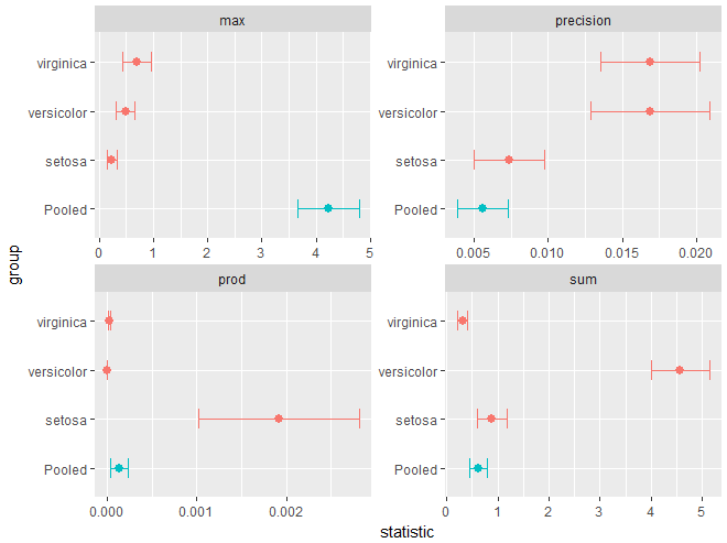
This gives something that can now be plotted, supposedly corresponding to the plot in the original question shown without error bars:

result %>% mutate(Pooled = group == "Pooled") %>%
    filter (term != "logdet") %>%
    ggplot(aes(y=statistic, x=group, color=Pooled)) +
    geom_point(size=2.5) +
    geom_errorbar(aes(ymin=statistic-2*std.error, 
                      ymax=statistic+2*std.error), width=0.4) +
    facet_wrap( ~ term, scales="free") +
    coord_flip() + guides(color=FALSE)

enter image description here

However, this "tidy plot" seems evidently WRONG. Theory says that the result for the Polled sample must in every case be intermediate between those for the separate groups, because it is in some sense a 'convex combination` over groups. Compare the plot below with that given in the original question. (It is possible that I did something wrong here, but I can't see a flaw.)

Jasso answered 3/8, 2017 at 15:32 Comment(0)

© 2022 - 2024 — McMap. All rights reserved.