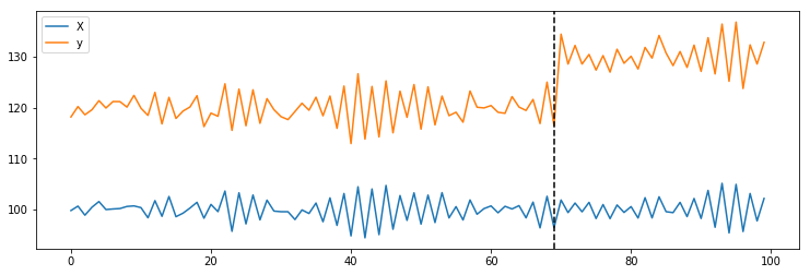
Simulating Time Series With Unobserved Components Model

After fitting a local level model using UnobservedComponents from statsmodels , we are trying to find ways to simulate new time series with the results. Something like:

import numpy as np
import statsmodels as sm
from statsmodels.tsa.statespace.structural import UnobservedComponents

np.random.seed(12345)
ar = np.r_[1, 0.9]
ma = np.array([1])
arma_process = sm.tsa.arima_process.ArmaProcess(ar, ma)

X = 100 + arma_process.generate_sample(nsample=100)
y = 1.2 * x + np.random.normal(size=100)
y[70:] += 10

plt.plot(X, label='X')
plt.plot(y, label='y')
plt.axvline(69, linestyle='--', color='k')
plt.legend();

ss = {}
ss["endog"] = y[:70]
ss["level"] = "llevel"
ss["exog"] = X[:70]

model = UnobservedComponents(**ss)
trained_model = model.fit()

Is it possible to use trained_model to simulate new time series given the exogenous variable X[70:]? Just as we have the arma_process.generate_sample(nsample=100), we were wondering if we could do something like:

trained_model.generate_random_series(nsample=100, exog=X[70:])

The motivation behind it is so that we can compute the probability of having a time series as extreme as the observed y[70:] (p-value for identifying the response is bigger than the predicted one).

[EDIT]

After reading Josef's and cfulton's comments, I tried implementing the following:

mod1 = UnobservedComponents(np.zeros(y_post), 'llevel', exog=X_post)
mod1.simulate(f_model.params, len(X_post))

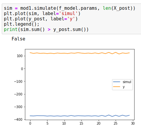
But this resulted in simulations that doesn't seem to track the predicted_mean of the forecast for X_post as exog. Here's an example:

While the y_post meanders around 100, the simulation is at -400. This approach always leads to p_value of 50%.

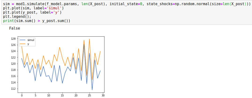
So when I tried using the initial_sate=0 and the random shocks, here's the result:

It seemed now that the simulations were following the predicted mean and its 95% credible interval (as cfulton commented below, this is actually a wrong approach as well as it's replacing the level variance of the trained model).

I tried using this approach just to see what p-values I'd observe. Here's how I compute the p-value:

samples = 1000
r = 0
y_post_sum = y_post.sum()
for _ in range(samples):
    sim = mod1.simulate(f_model.params, len(X_post), initial_state=0, state_shocks=np.random.normal(size=len(X_post)))
    r += sim.sum() >= y_post_sum
print(r / samples)

For context, this is the Causal Impact model developed by Google. As it's been implemented in R, we've been trying to replicate the implementation in Python using statsmodels as the core to process time series.

We already have a quite cool WIP implementation but we still need to have the p-value to know when in fact we had an impact that is not explained by mere randomness (the approach of simulating series and counting the ones whose summation surpasses y_post.sum() is also implemented in Google's model).

In my example I used y[70:] += 10. If I add just one instead of ten, Google's p-value computation returns 0.001 (there's an impact in y) whereas in Python's approach it's returning 0.247 (no impact).

Only when I add +5 to y_post is that the model returns p_value of 0.02 and as it's lower than 0.05, we consider that there's an impact in y_post.

I'm using python3, statsmodels version 0.9.0

[EDIT2]

After reading cfulton's comments I decided to fully debug the code to see what was happening. Here's what I found:

When we create an object of type UnobservedComponents, eventually the representation of the Kalman Filter is initiated. As default, it receives the parameter initial_variance as 1e6 which sets the same property of the object.

When we run the simulate method, the initial_state_cov value is created using this same value:

initial_state_cov = (
        np.eye(self.k_states, dtype=self.ssm.transition.dtype) *
        self.ssm.initial_variance
    )

Finally, this same value is used to find initial_state:

initial_state = np.random.multivariate_normal(
    self._initial_state, self._initial_state_cov)

Which results in a normal distribution with 1e6 of standard deviation.

I tried running the following then:

mod1 = UnobservedComponents(np.zeros(len(X_post)), level='llevel', exog=X_post, initial_variance=1)
sim = mod1.simulate(f_model.params, len(X_post))
plt.plot(sim, label='simul')
plt.plot(y_post, label='y')
plt.legend();
print(sim.sum() > y_post.sum())

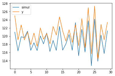
Which resulted in:

I tested then the p-value and finally for a variation of +1 in y_post the model now is identifying correctly the added signal.

Still, when I tested with the same data that we have in R's Google package the p-value was still off. Maybe it's a matter of further tweaking the input to increase its accuracy.

coef std err z P>|z| [0.025 0.975] ------------------------------------------------------------------------------------ sigma2.irregular 0.9278 0.194 4.794 0.000 0.548 1.307 sigma2.level 0.0021 0.008 0.270 0.787 -0.013 0.018 beta.x1 1.1882 0.058 20.347 0.000 1.074 1.303

mod1 = UnobservedComponents(np.zeros(y_post), 'llevel', exog=X_post) initial_state = np.random.multivariate_normal( f_model.predicted_state[..., -1], f_model.predicted_state_cov[..., -1]) mod1.simulate(f_model.params, len(X_post), initial_state=initial_state)

Recommended topics

Hot tags