With ResNet50 the validation accuracy and loss is not changing

I am trying to do image recognition with ResNet50 in Python (keras). I tried to do the same task with VGG16, and I got some results like these (which seem okay to me): resultsVGG16 . The training and validation accuracy/loss functions are getting better with each step, so the network must learn.

However, with ResNet50 the training functions are betting better, while the validation functions are not changing: resultsResNet

I've used the same code and data in both of the times, only the model is changed.

So what are the reasons of ResNet50 learning only on the training data?

My ResNet model looks like this:

'''python

model = Sequential()
base_model = VGG16(weights='imagenet', include_top=False,input_shape= 
(image_size,image_size,3))
for layer in base_model.layers[:-4]:
    layer.trainable=False

model.add(base_model)
model.add(Flatten())
model.add(Dense(256, activation='relu'))
model.add(Dropout(0.4))
model.add(Dense(NUM_CLASSES, activation='softmax'))

The VGG is very similar:

model = Sequential()
base_model = ResNet50(include_top=False, weights='imagenet', input_shape= 
(image_size,image_size,3))
for layer in base_model.layers[:-8]:
     layer.trainable=False

model.add(base_model)
model.add(Flatten())
model.add(Dense(256, activation='relu'))
model.add(Dropout(0.4))
model.add(Dense(NUM_CLASSES, activation='softmax'))

There is no mistake in your Model but this might be the issue with ResNet as such, because there are many issues raised, 1,2,3, in Github and Stack Overflow, already regarding this Pre-Trained Model.

Having said that, I found out a workaround, which worked for me, and hopefully works for you as well.

Workaround was to replace the Data Augmentation step,

Train_Datagen = ImageDataGenerator(rescale=1./255,  rotation_range=40, width_shift_range=0.2,
    height_shift_range=0.2, brightness_range=(0.2, 0.7), shear_range=45.0, zoom_range=60.0,
    horizontal_flip=True, vertical_flip=True)

Val_Datagen = ImageDataGenerator(rescale=1./255,  rotation_range=40, width_shift_range=0.2,
    height_shift_range=0.2, brightness_range=(0.2, 0.7), shear_range=45.0, zoom_range=60.0,
    horizontal_flip=True, vertical_flip=True)

with tf.keras.applications.resnet.preprocess_input, as shown below:

Train_Datagen = ImageDataGenerator(dtype = 'float32', preprocessing_function=tf.keras.applications.resnet.preprocess_input)
Val_Datagen = ImageDataGenerator(dtype = 'float32', preprocessing_function=tf.keras.applications.resnet.preprocess_input)

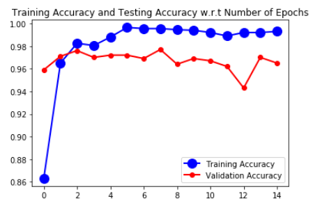
By modifying the Data Augmentation as shown above, my Validation Accuracy, which got stuck at 50% increased gradually up to 97%. Reason for this might be that ResNet might expect specific Pre-Processing Operations (not quite sure).

Complete working code which resulted in more than 95% of both Train and Validation Accuracy (for Cat and Dog Dataset) using ResNet50 is shown below:

import tensorflow as tf
from tensorflow.keras.applications import ResNet50
import os
import numpy as np
from keras.preprocessing.image import ImageDataGenerator
from tensorflow.keras.layers import Dense, Dropout, Flatten
from tensorflow.keras.optimizers import Adam
from tensorflow.keras.models import Sequential

# The Convolutional Base of the Pre-Trained Model will be added as a Layer in this Model
Conv_Base = ResNet50(include_top = False, weights = 'imagenet', input_shape = (150,150, 3))

for layer in Conv_Base.layers[:-8]:
    layer.trainable = False

model = Sequential()
model.add(Conv_Base)
model.add(Flatten())
model.add(Dense(units = 256, activation = 'relu'))
model.add(Dropout(0.5))
model.add(Dense(units = 1, activation = 'sigmoid'))

model.summary()

base_dir = 'Deep_Learning_With_Python_Book/Dogs_Vs_Cats_Small'
if os.path.exists(base_dir):    
    train_dir = os.path.join(base_dir, 'train')
    validation_dir = os.path.join(base_dir, 'validation')
    test_dir = os.path.join(base_dir, 'test')
else:
    print("The Folder, {}, doesn't exist'".format(base_dir))

batch_size = 20

Train_Datagen = ImageDataGenerator(dtype = 'float32', preprocessing_function=tf.keras.applications.resnet.preprocess_input)
Val_Datagen = ImageDataGenerator(dtype = 'float32', preprocessing_function=tf.keras.applications.resnet.preprocess_input)

train_gen = Train_Datagen.flow_from_directory(directory = train_dir, target_size = (150,150), 
                                       batch_size = batch_size, class_mode = 'binary')

val_gen = Val_Datagen.flow_from_directory(directory = validation_dir, target_size = (150,150), 
                                       batch_size = batch_size, class_mode = 'binary')

epochs = 15
Number_Of_Training_Images = train_gen.classes.shape[0]
steps_per_epoch = Number_Of_Training_Images/batch_size

model.compile(optimizer = 'Adam', loss = 'binary_crossentropy', metrics = ['accuracy'])

history = model.fit(train_gen, epochs = epochs, 
                    #batch_size = batch_size,
                    validation_data = val_gen, steps_per_epoch = steps_per_epoch)

import matplotlib.pyplot as plt

train_acc = history.history['accuracy']
val_acc = history.history['val_accuracy']
train_loss = history.history['loss']
val_loss = history.history['val_loss']
No_Of_Epochs = range(epochs)

plt.plot(No_Of_Epochs, train_acc, marker = 'o', color = 'blue', markersize = 12, 
                 linewidth = 2, label = 'Training Accuracy')
plt.plot(No_Of_Epochs, val_acc, marker = '.', color = 'red', markersize = 12, 
                 linewidth = 2, label = 'Validation Accuracy')

plt.title('Training Accuracy and Testing Accuracy w.r.t Number of Epochs')

plt.legend()

plt.figure()

plt.plot(No_Of_Epochs, train_loss, marker = 'o', color = 'blue', markersize = 12, 
                 linewidth = 2, label = 'Training Loss')
plt.plot(No_Of_Epochs, val_acc, marker = '.', color = 'red', markersize = 12, 
                 linewidth = 2, label = 'Validation Loss')

plt.title('Training Loss and Testing Loss w.r.t Number of Epochs')

plt.legend()

plt.show()

Metrics are shown in the below graph,

Recommended topics

Hot tags