Forecasting with statsmodels

Question

I have a .csv file containing a 5-year time series, with hourly resolution (commoditiy price). Based on the historical data, I want to create a forecast of the prices for the 6th year.

I have read a couple of articles on the www about these type of procedures, and I basically based my code on the code posted there, since my knowledge in both Python (especially statsmodels) and statistic is at most limited.

Those are the links, for those who are interested:

http://www.seanabu.com/2016/03/22/time-series-seasonal-ARIMA-model-in-python/

http://www.johnwittenauer.net/a-simple-time-series-analysis-of-the-sp-500-index/

First of all, here is a sample of the .csv file. Data is displayed with monthly resolution in this case, it is not real data, just randomly choosen numbers to give an example here (in which case I hope one year is enough to be able to develop a forecast for the 2nd year; if not, full csv file is available):

              Price
2011-01-31    32.21
2011-02-28    28.32
2011-03-31    27.12
2011-04-30    29.56
2011-05-31    31.98
2011-06-30    26.25
2011-07-31    24.75
2011-08-31    25.56
2011-09-30    26.68
2011-10-31    29.12
2011-11-30    33.87
2011-12-31    35.45

My current progress is as follows:

After reading the input file and setting the date column as datetime index, the follwing script was used to develop a forecast for the available data

model = sm.tsa.ARIMA(df['Price'].iloc[1:], order=(1, 0, 0))  
results = model.fit(disp=-1)  
df['Forecast'] = results.fittedvalues  
df[['Price', 'Forecast']].plot(figsize=(16, 12))  

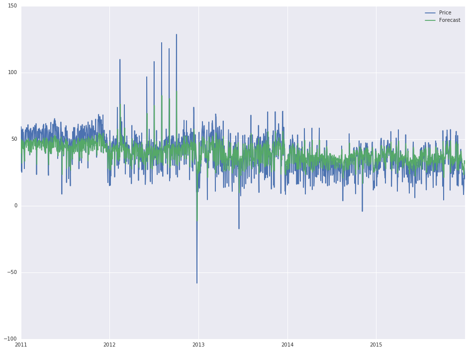
,which gives the following output:

Now, as I said, I ain't got no statistic skills and I have little to no idea how I got to this output (basically, changing the order attribute inside the first line changes the output), but the 'actual' forecast looks quite good and I would like to extend it for another year (2016).

In order to do that, additional rows are created in the dataframe, as follows:

start = datetime.datetime.strptime("2016-01-01", "%Y-%m-%d")
date_list = pd.date_range('2016-01-01', freq='1D', periods=366)
future = pd.DataFrame(index=date_list, columns= df.columns)
data = pd.concat([df, future])

Finally, when I use the .predict function of statsmodels:

data['Forecast'] = results.predict(start = 1825, end = 2192, dynamic= True)  
data[['Price', 'Forecast']].plot(figsize=(12, 8))

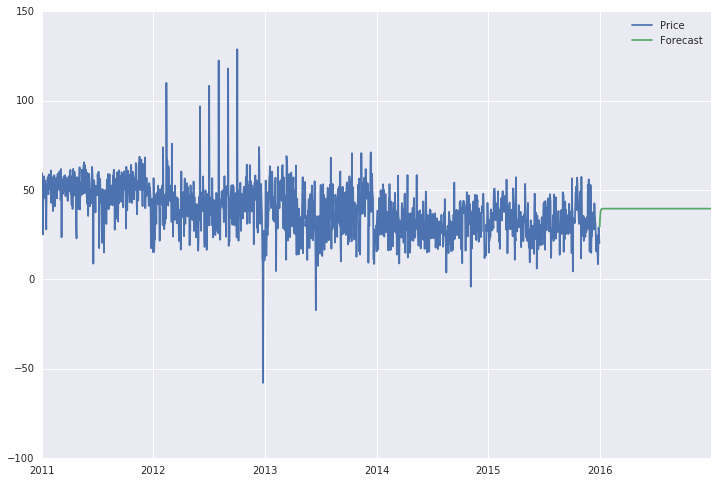
what I get as forecast is a straight line (see below), which doesn't seem at all like a forecast. Moreover, if I extend the range, which now is from the 1825th to 2192nd day (year of 2016), to the whole 6 year timespan, the forecast line is a straight line for the entire period (2011-2016).

I have also tried to use the 'statsmodels.tsa.statespace.sarimax.SARIMAX.predict' method, which accounts for a seasonal variation (which makes sense in this case), but I get some error about 'module' has no attribute 'SARIMAX'. But this is secondary problem, will get into more detail if needed.

Somewhere I am losing grip and I have no idea where. Thanks for reading. Cheers!

Assegai

I have a similar problem. Were you able to solve it? Thanks – Brodie

no, I haven't solved it. I dropped it at some point, due to some interruption in my work and never gor back to this.. – Assegai

Answer 1

It sounds like you are using an older version of statsmodels that does not support SARIMAX. You'll want to install the latest released version 0.8.0 see http://statsmodels.sourceforge.net/devel/install.html.

I'm using Anaconda and installed via pip.

pip install -U statsmodels

The results class from the SARIMAX model have a number of useful methods including forecast.

data['Forecast'] = results.forecast(100)

Will use your model to forecast 100 steps into the future.

Famous

if you want to forecast out of sample, and you have exogenous variables, you have first to provide forecasts of these (which you may not have). – Reputation

Shout out to Geoff D and fccoelho. The language in the documentation was confusing. Seeing this finally made it make sense. – Weldon

Answer 2

ARIMA(1,0,0) is a one period autoregressive model. So it's a model that follows this formula:

What that means is that the value in time period t is equal to some constant (phi_0) plus a value determined by fitting the ARMA model (phi_1) multiplied by the value in the prior period r_(t-1), plus a white noise error term (a_t).

Your model only has a memory of 1 period, so the current prediction is entirely determined by the 1 value of the prior period. It's not a very complex model; it's not doing anything fancy with all the prior values. It's just taking yesterday's price, multiplying it by some value and adding a constant. You should expect it to quickly go to equilibrium and then stay there forever.

The reason why the forecast in the top picture looks so good is that it is just showing you hundreds of 1 period forecasts that are starting fresh with each new period. It's not showing a long period prediction like you probably think it is.

Looking at the link you sent:

http://www.johnwittenauer.net/a-simple-time-series-analysis-of-the-sp-500-index/

read the section where he discusses why this model doesn't give you what you want.

"So at first glance it seems like this model is doing pretty well. But although it appears like the forecasts are really close (the lines are almost indistinguishable after all), remember that we used the un-differenced series! The index only fluctuates a small percentage day-to-day relative to the total absolute value. What we really want is to predict the first difference, or the day-to-day moves. We can either re-run the model using the differenced series, or add an "I" term to the ARIMA model (resulting in a (1, 1, 0) model) which should accomplish the same thing. Let's try using the differenced series."

To do what you're trying to do, you'll need to do more research into these models and figure out how to format your data, and what model will be appropriate. The most important thing is knowing what information you believe is contained in the data you're feeding into the model. What your model currently is trying to do is say, "Today the price is $45. What will the price be tomorrow?" That's it. It doesn't have any information about momentum, volatility, etc. That's not much to go off.

Roundtree

Answer 3

try set dynamic = False when predicting

Sitsang

can you please elaborate on your answer instead of providing one line answer. It does. not help the OP to troubleshoot. – Edinburgh