I will give three procedures, each of which is a marginalized random intercept model (MRIM). These MRIMs have coefficients with marginal logistic interpretations and are of smaller magnitude than the GEE:
| Model | (Intercept) |  power |  LogL  |
|-------|-------------|--------|--------|
| `L_N` |       -1.050| 0.00267|  -270.1|
| `LLB` |       -0.668| 0.00343|  -273.8|
| `LPN` |       -1.178| 0.00569|  -266.4|
compared to a glm that doesn't account for any correlation, for reference:
| Model | (Intercept) |  power |  LogL  |
|-------|-------------|--------|--------|
|  strt |       -0.207| 0.00216|  -317.1|
A marginalized random intercept model (MRIM) is worth exploring because you want a marginal model with exchangeable correlation structure for the clustered data, and that is the type of structure MRIMs exhibit.
The code (especially R script with comments) and PDFs for literature are in the GITHUB repo. I detail the code and literature down below.
The concept of MRIM has been around since 1999, and some background reading on this is in the GITHUB repo. I suggest reading Swihart et al 2014 first because it reviews the other papers.
In chronological order --
L_N Heagerty (1999): the approach fits a random intercept logistic model with a normally distributed random intercept. The trick is that the predictor in the random intercept model is nonlinearly parameterized with marginal coefficients so that the resulting marginal model has a marginal logistic interpretation. Its code is the lnMLE R package (not on CRAN, but on Patrick Heagerty's website here). This approach is denoted L_N in the code to indicate logit (L) on the marginal, no interepretation on conditional scale (_) and a normally (N) distributed random intercept.
LLB Wang & Louis (2003): the approach fits a random intercept logistic model with a bridge distributed random intercept. Unlike Heagerty 1999 where the trick is nonlinear-predictor for the random intercept model, the trick is a special random effects distribution (the bridge distribution) that allows both the random intercept model and the resulting marginal model to have a logistic interpretation. Its code is implemented with gnlmix4MMM.R (in the repo) which uses rmutil and repeated R packages. This approach is denoted LLB in the code to indicate logit (L) on the marginal, logit (L) on the conditional scale and a bridge (B) distributed intercept.
LPN Caffo and Griswold (2006): the approach fits a random intercept probit model with a normally distributed random intercept, whereas Heagerty 1999 used a logit random intercept model. This substitution makes computations easier and still yields a marginal logit model. Its code is implemented with gnlmix4MMM.R (in the repo) which uses rmutil and repeated R packages. This approach is denoted LPN in the code to indicate logit (L) on the marginal, probit (P) on the conditional scale and a normally (N) distributed intercept.
Griswold et al (2013): another review / practical introduction.
Swihart et al 2014: This is a review paper for Heagerty 1999 and Wang & Louis 2003 as well as others and generalizes the MRIM method. One of the most interesting generalizations is allowing the logistic CDF (equivalently, logit link) in both the marginal and conditional models to instead be a stable distribution that approximates a logistic CDF. Its code is implemented with gnlmix4MMM.R (in the repo) which uses rmutil and repeated R packages. I denote this SSS in the R script with comments to indicate stable (S) on the marginal, stable (S) on the conditional scale and a stable (S) distributed intercept. It is included in the R script but not detailed in this post on SO.
Prep
#code from OP Question: edit `data` to `d`
require(geepack)
d = read.csv(url("http://folk.uio.no/mariujon/data.csv"))
fit = geeglm(moden ~ 1 + power, id = defacto, data=d, corstr = "exchangeable", family=binomial)
summary(fit)
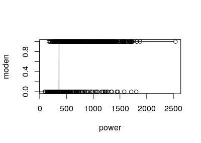
plot(moden ~ power, data=d)
x = 0:2500
y = predict(fit, newdata=data.frame(power = x), type="response" )
lines(x,y)
#get some starting values from glm():
strt <- coef(glm(moden ~  power, family = binomial, data=d))
strt
#I'm so sorry but these methods use attach()
attach(d)
L_N Heagerty (1999)
# marginally specifies a logit link and has a nonlinear conditional model
# the following code will not run if lnMLE is not successfully installed.
# See https://faculty.washington.edu/heagerty/Software/LDA/MLV/
library(lnMLE)
L_N <- logit.normal.mle(meanmodel = moden ~ power,
                        logSigma= ~1,
                        id=defacto,
                        model="marginal",
                        data=d,
                        beta=strt,
                        r=10)
print.logit.normal.mle(L_N)
Prep for LLB and LPN
library("gnlm")
library("repeated")
source("gnlmix4MMM.R") ## see ?gnlmix; in GITHUB repo
y <- cbind(d$moden,(1-d$moden))
LLB Wang and Louis (2003)
LLB  <- gnlmix4MMM(y = y,
                   distribution = "binomial",
                   mixture = "normal",
                   random = "rand",
                   nest = defacto,
                   mu = ~ 1/(1+exp(-(a0 + a1*power)*sqrt(1+3/pi/pi*exp(pmix)) - sqrt(1+3/pi/pi*exp(pmix))*log(sin(pi*pnorm(rand/sqrt(exp(pmix)))/sqrt(1+3/pi/pi*exp(pmix)))/sin(pi*(1-pnorm(rand/sqrt(exp(pmix))))/sqrt(1+3/pi/pi*exp(pmix)))))),
                   pmu = c(strt, log(1)),
                   pmix = log(1))

print("code: 1 -best 2-ok 3,4,5 - problem")
LLB$code
print("coefficients")
LLB$coeff
print("se")
LLB$se
LPN Caffo and Griswold (2006)
LPN  <- gnlmix4MMM(y = y,
                   distribution = "binomial",
                   mixture = "normal",
                   random = "rand",
                   nest = defacto,
                   mu = ~pnorm(qnorm(1/(1+exp(-a0 - a1*power)))*sqrt(1+exp(pmix)) + rand),
                   pmu = c(strt, log(1)),
                   pmix = log(1))

print("code: 1 -best 2-ok 3,4,5 - problem")
LPN$code
print("coefficients")
LPN$coeff
print("se")
LPN$se
coefficients from 3 approaches:
rbind("L_N"=L_N$beta, "LLB" = LLB$coefficients[1:2], "LPN"=LPN$coefficients[1:2])
max log likelihood for 3 models:
rbind("L_N"=L_N$logL, "LLB" = -LLB$maxlike, "LPN"=-LPN$maxlike)


MCMCglmmorblmepackages), but it will fit the conditional rather than the marginal model ... I don't know offhand how to implement shrinkage in the GEE framework, or whether someone has already done it. – Burkes(Intercept)and 0.003 forpower. Is there interest in my writing it up? – Stumpf