Several points for consideration.
1 - Optimal place for annotation purposes within a polygon
In an ideal world, every polygon is similar to a circle, and its centre is the best place to position a text label (e.g. Texas). In reality, map regions come in all sorts of shapes, & may not even be in one piece (e.g. Michigan). The mathematical mean / median point may be on the edge or outside the polygon (e.g. Florida).
R isn't going to be that great at trying to figure out these complications. I'd use a GIS software instead.
However, if your use case is US, the state.vbm.center dataset already comes with a pretty good set of default coordinates. Its help file states:
state.vbm.center are coordinates of the state centers for annotation
purposes.
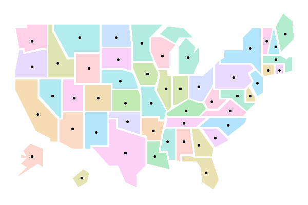
Let's take a look at where these points are:
#data
mapbase <- map_data("state.vbm")
data(state.vbm.center)

cnames <- state.vbm.center %>% as.data.frame() %>%
  mutate(region = unique(mapbase$region))

#actual plotting
ggplot()+
  geom_polygon( data=mapbase,
                aes(long, lat, group = region, fill = region),
                alpha = 0.3) +
  coord_fixed() + theme_void() +
  geom_point(data = cnames,
             aes(x, y)) +
  scale_fill_discrete(guide = F)
![center location]()
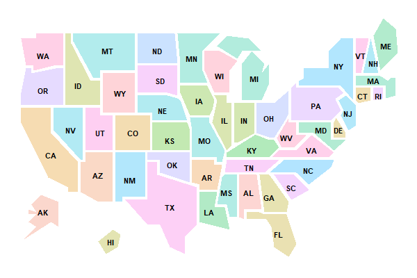
That's not too shabby. If all you need to label are state names, this should suffice:
cnames$abb <- state.abb

ggplot()+
  geom_polygon( data=mapbase,
                aes(long, lat, group = region, fill = region),
                alpha = 0.3) +
  coord_fixed() + theme_void() +
  geom_text(data=cnames,
            aes(x, y , label = abb),
            color= "black", size=3, fontface = 2,
            hjust = 0.5, vjust = 0.5) + #central alignment
  scale_fill_discrete(guide = F)
![abbreviated names]()
2 - Fitting long labels into tight spaces
It's very well fitting short labels within map polygons, but if you want to include more information (full name of each state, birth rate, crime rate, unemployment rate, education level, income range, population density, proportion of people who voted in the last election, ...), eventually you'll start to run out of space in the smaller / more weirdly shaped polygons.
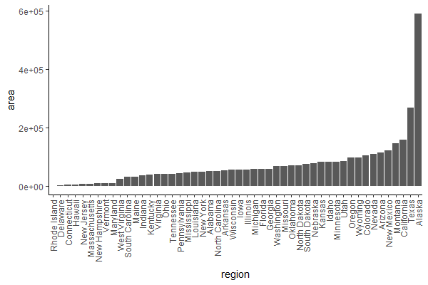
A dual approach can be adopted at this point, keeping information within the larger polygons, & placing the smaller polygons separately on one side like a partial legend. For US states, state area is part of the standard datasets package, which saves us the trouble of calculating it:
# incorporate area information & identify small area states
cnames$area <- state.area
ggplot(cnames %>%
         mutate(region = factor(region, levels = region[order(area)])),
       aes(x = region, y = area)) + geom_col() +
  theme_classic() +
  theme(axis.text.x = element_text(angle = 90, vjust = 0.5, hjust = 1))

# the first 7 states (up to Maryland) are noticeably smaller than the rest
![sorted by area size]()
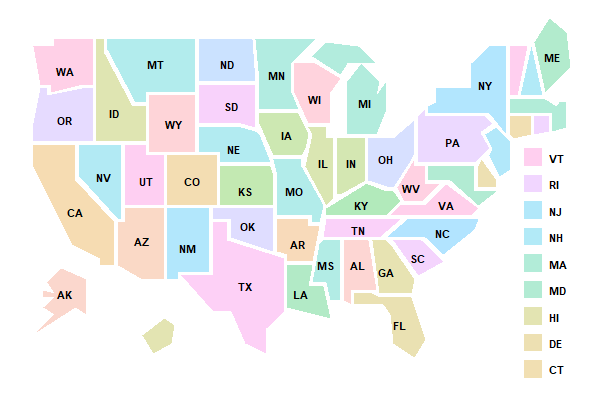
Pick some nice empty area on your map for the small states. I decided to align them vertically in 1 column at longitude = 140, & latitude ranging from 0 to 60:
library(tidyr)

legend.states <- cnames$region[which(cnames$area <= 10577)]
legend.states <- as.data.frame(legend.states)
legend.states$long1 <- 140
legend.states$lat1 <- seq(0, 60, length.out = nrow(legend.states))
legend.states <- legend.states %>%
  mutate(long2 = long1 + 5, lat2 = lat1) %>%
  mutate(long3 = long2, lat3 = lat2 - 5) %>%
  mutate(long4 = long1, lat4 = lat3) %>%
  mutate(long5 = long1, lat5 = lat1) %>%
  gather(k, v, -legend.states) %>%
  mutate(order = as.integer(substring(k, nchar(k))),
         k = gsub("[0-9]", "", k)) %>%
  spread(k, v) %>%
  rename(region = legend.states) %>%
  mutate(group = mapbase$group[match(region, mapbase$region)]) %>%
  select(long, lat, group, order, region) %>%
  mutate(subregion = NA)

# add legend polygons to the original polygon dataset
mapbase2 <- rbind(mapbase, legend.states)
Change the annotation coordinates for these small states, such that they are aligned to the legend box positions:
cnames2 <- left_join(cnames,
                     legend.states %>% filter(order %in% c(1, 4)) %>%
                       group_by(region) %>%
                       summarise(long = mean(long) + 7,
                                 lat = mean(lat))) %>%
  mutate(x = coalesce(long, x),
         y = coalesce(lat, y),
         hjust = ifelse(is.na(lat), 0.5, 0))
# left alignment (hjust=0) for small state text, central alignment (hjust=0.5) otherwise.
Put everything together:
ggplot()+
  geom_polygon( data=mapbase2,
                aes(long, lat, group = region, fill = region),
                alpha = 0.3) +
  coord_fixed() + theme_void() +
  geom_text(data=cnames2,
            aes(x, y , label = abb, hjust = hjust),
            size=3, fontface = 2,
            vjust = 0.5) +
  scale_fill_discrete(guide = F)
![legend box]()
(Note: for longer text, you'll probably need to increase the x-axis limits as well, and/or insert line breaks.)
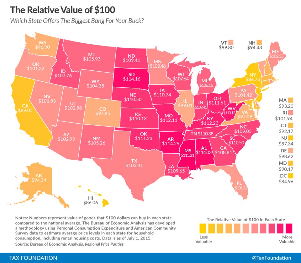 (image from http://www.businessinsider.com/map-what-100-is-actually-worth-in-your-state-2015-7?IR=T)
