Plotting shape files loaded using read.shp with ggplot2
Asked Answered
Y

1

1

I would like to plot a shape file loaded using read.shp from the fastshp package. However, the read.shp function returns a list of list and not a data.frame. I'm unsure which part of the list I need to extract to obtain the correctly formatted data.frame object. This exact question has been asked on stack overflow already, however, the solution no longer seems to work (solution was from > 7 years ago). Any help is much appreciated.

remotes::install_github("s-u/fastshp") #fastshp not on CRAN
library(ggplot2);library(fastshp)

temp <- tempfile()
temp2 <- tempfile()
download.file("https://www2.census.gov/geo/tiger/TIGER2017/COUNTY/tl_2017_us_county.zip",temp)
unzip(zipfile = temp, exdir = temp2)
shp <- list.files(temp2, pattern = ".shp$",full.names=TRUE) %>% read.shp(.)

shp is a list of lists containing a plethora of information. I tried the following solution from the SO posted earlier, but to no avail:

shp.list <- sapply(shp, FUN = function(x) Polygon(cbind(lon = x$x, lat = x$y))) #throws an error here cbind(lon = x$x, lat = x$y) returns NULL
shp.poly <- Polygons(shp.list, "area")
shp.df <- fortify(shp.poly, region = "area")

I also tried the following:

shp.list <- sapply(shp, FUN = function(x) do.call(cbind, x[c("id","x","y")])) #returns NULL value here...
shp.df <- as.data.frame(do.call(rbind, shp.list))

Updated: Still no luck but closer:

file_shp<-list.files(temp2, pattern = ".shp$",full.names=TRUE) %>%
  read.shp(., format = c("table"))

ggplot() + 
geom_polygon(data = file_shp, aes(x = x, y = y, group = part), 
             colour = "black", fill = NA)

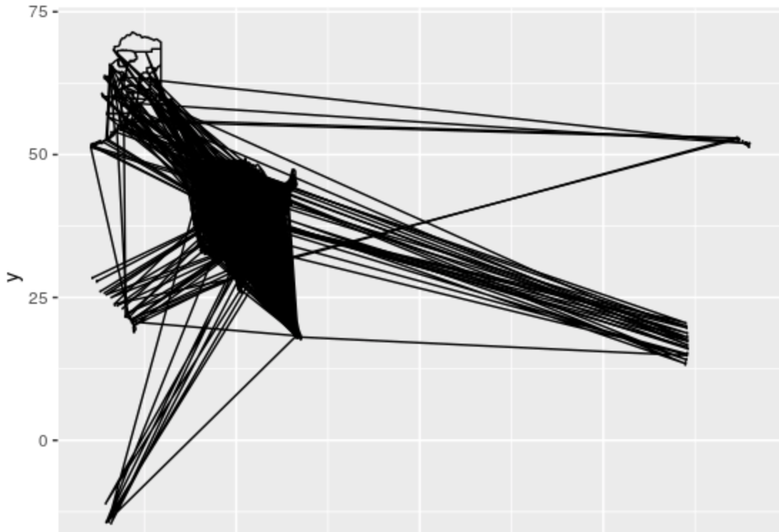
enter image description here

Looks like the projection is off. I'm not sure how to order the data to map correctly, also not sure how to read in the CRS data. Tried the following to no avail:

file_prj<-list.files(temp2, pattern = ".prj$",full.names=TRUE) %>%
  proj4string(.)
Yellowknife answered 14/1, 2020 at 20:4 Comment(10)
Any interest in trying sf? It converts between formats well and there's a geom_sf for plotting sf objectsJacquerie
@Camille if it doesn't rely on rgdal, I'm open to it. I'll give it a shot!Yellowknife
Unfortunately, sf relies on the units package, which like rgdal, requires additional software to be installed, which I lack the ability to do. So back to square one...Yellowknife
Oh, bummer. Can you add an example somehow that folks could reproduce? Maybe with shapefiles that ship with one of the packages you can use?Jacquerie
@Camille just updated using a random shapefile from the net. thanks!Yellowknife
@CyrusMohammadian I was following your code, but R studio crashes when I ran shp <- list.files(temp2, pattern = ".shp$",full.names=TRUE) %>% read.shp(.). I wonder what is causing this issue.Conchiferous
@Conchiferous thank you for running the code. Yea, not sure.Yellowknife
@CyrusMohammadian I just posted what I investigated. Have a look. I hope this guides you through.Conchiferous
@Conchiferous this is fantastic. You really dug deep on this and that's much appreciated.Yellowknife
@CyrusMohammadian Pleasure to help you. I had a chance to learn how to draw maps in another way. :) I hope you can keep rolling using this idea.Conchiferous
C
1

I tried to use the census data you have in your script. However, R Studio somehow kept crashing when I applied read.shp() to the polygon data. Hence, I decided to use the example from the help page of read.shp(), which is also census data. I hope you do not mind. It took some time to figure out how to draw a map with class shp. Let me explain what I went through step by step.

This part is from the help page. I am basically getting shapefile and importing it as shp object.

# Census 2010 TIGER/Line(TM) state shapefile
library(fastshp)
fn <- system.file("shp", "tl_2010_us_state10.shp.xz", package="fastshp")
s <- read.shp(xzfile(fn, "rb"))

Let's check how this object, s is like. It contains 52 lists. In each list, there are six vectors. ID is a unique integer to represent a state. x is longitude and y is latitude. The nasty part was parts. In this example below, there is only one number, which means there is one polygon only in this state. But some other lists (states) have multiple numbers. These numbers are basically indices which indicate where new polygons begin in the data.

#> str(s)
#List of 52
# $ :List of 6
#  ..$ id   : int 1
#  ..$ type : int 5
#  ..$ box  : num [1:4] -111 41 -104 45
#  ..$ parts: int 0
#  ..$ x    : num [1:9145] -109 -109 -109 -109 -109 ...
#  ..$ y    : num [1:9145] 45 45 45 45 45 ...

Here is the one for Alaska. As you see there are some numbers in parts These numbers indicate where new polygon data begin. Alaksa has many small islands. Hence they needed to indicate different polygons in the data with this information. We will come back to this later when we create data frames.

#List of 6
# $ id   : int 18
# $ type : int 5
# $ box  : num [1:4] -179.2 51.2 179.9 71.4
# $ parts: int [1:50] 0 52 88 127 175 207 244 306 341 375 ...
# $ x    : num [1:14033] 177 177 177 177 177 ...
# $ y    : num [1:14033] 52.1 52.1 52.1 52.1 52.1 ...

What we need is the following. For each list, we need to extract longitude (i.e., x), latitude (i.e., y), and id in order to create a data fame for one state. In addition, we need to use parts so that we can indicate all polygons with unique IDs. We need to crate a new group variable, which contains unique ID value for each polygon. I used findInterval() which takes indices to create a group variable. One tricky part was that we need to use left.open = TRUE in findInterval() in order to create a group variable. (This gave me some hard time to figure out what was going on.) This map_dfr() part handles the job I just described.

library(tidyverse)

map_dfr(.x = s,
        .f = function(mylist){

                temp <- data.frame(id = mylist$id,
                                   lon = mylist$x,
                                   lat = mylist$y)
                ind <- mylist$parts

                out <- mutate(temp,
                              subgroup = findInterval(x = 1:n(), vec = ind, left.open = TRUE),
                              group = paste(id, subgroup, sep = "_"))
                return(out)

                }) -> test

Once we have test, we have another job. Some longitude points of Alaska stay in positive numbers (e.g., 179.85). As long as we have numbers like this, ggplot2 draws funny long lines, which you can see even in your example. What we need is to convert these positive numbers to negative ones so that ggplot2 can draw a proper map.

mutate(test,
       lon = if_else(lon > 0, lon * -1, lon)) -> out

By this time, out looks like this.

  id       lon      lat subgroup group
1  1 -108.6213 45.00028        1   1_1
2  1 -108.6197 45.00028        1   1_1
3  1 -108.6150 45.00031        1   1_1
4  1 -108.6134 45.00032        1   1_1
5  1 -108.6133 45.00032        1   1_1
6  1 -108.6130 45.00032        1   1_1

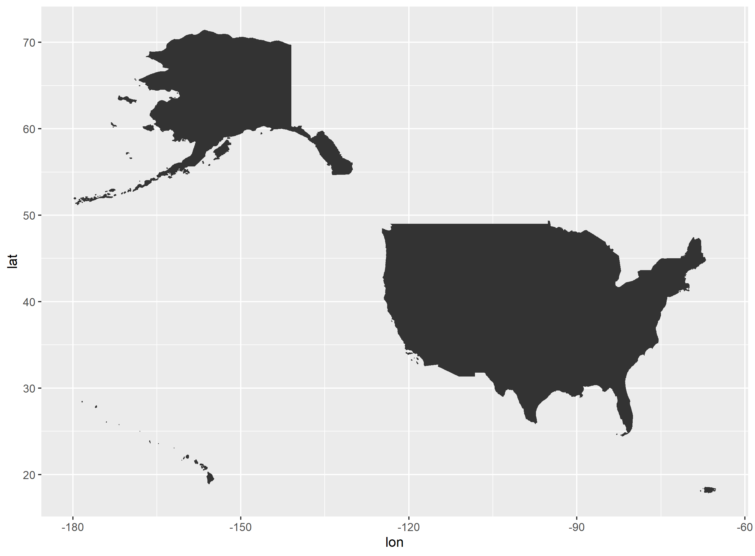
Now we are ready to draw a map.

ggplot() +
geom_polygon(data = out, aes(x = lon, y = lat, group = group))

enter image description here

Conchiferous answered 15/1, 2020 at 3:30 Comment(0)

© 2022 - 2024 — McMap. All rights reserved.