Plotting both state AND county boundaries on same map using plot_usmap from usmap package in R

Question

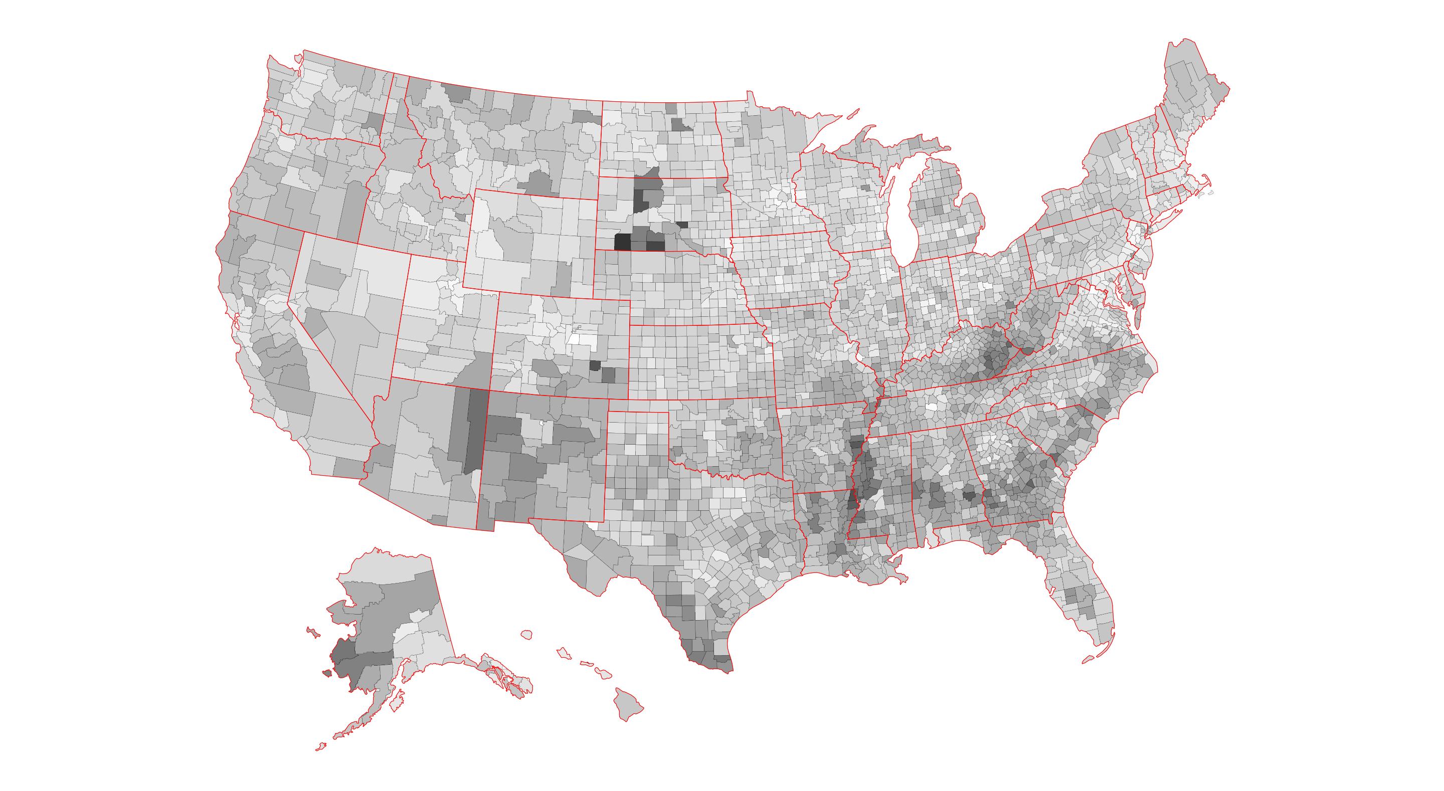
I would like to create a map of the US showing both state and county boundaries (i.e. state boundaries in a different color). I typically do this using either shape files that I import or using ggplot2's map_data function. However, I face three obstacles.

1) I cannot install gdal and geos in my computing environment so that precludes the use of any shape files or GeoJSON files (my attempts to map county level shape files loaded using fastshp have not been successful but I'm open to any solution that can reproduce the map below but with state boundaries included).

2) I need to include Hawaii and Alaska, so that excludes the use of map_data from ggplot2.

3) I need the map to include both state AND county boundaries, which makes the use of usmap package problematic as its a wrapper function for ggplot2 but without the ease and general ability to customize to the level of a raw ggplot2 object.

4) Also, cannot make use of sf package bc it has a non R library dependency (units package depends on C library libudunits2).

What I need: A map that can project Alaska and Hawaii and display state and county boundaries using contrasting colors and I need to accomplish all this without resorting to any packages that rely on rgeos, rgdal, and/or units.

What I've tried thus far plot_usmap from the usmap package:

library(dplyr)
library(stringr)
library(ggplot2)
library(usmap)
library(mapproj)
devtools::install_github("wmurphyrd/fiftystater")
library(fiftystater)

county_data<-read.csv("https://www.ers.usda.gov/webdocs/DataFiles/48747/PovertyEstimates.csv?v=2529") %>% #
  filter(Area_name != "United States") %>%
  select(FIPStxt, Stabr, Area_name, PCTPOVALL_2017) %>%
  rename(fips = FIPStxt)
crimes <- data.frame(state = tolower(rownames(USArrests)), USArrests)
state_map <- map_data("state")

plot_usmap(data = county_data, values = "PCTPOVALL_2017", color = "white") + 
  geom_map(data = crimes, aes(map_id = state), map = fifty_states, color= "red") + 
  geom_path(data = state_map, aes(x =long , y=lat), color= "red")+
  expand_limits(x = fifty_states$long, y = fifty_states$lat) +
  theme(legend.position = "none") +
  theme_map() #no go

plot_usmap(data = county_data, values = "PCTPOVALL_2017", color = "white") + 
  geom_map(data = crimes, aes(map_id = state), map = fifty_states, color= "red") + 
  expand_limits(x = fifty_states$long, y = fifty_states$lat) +
  theme(legend.position = "none") +
  theme_map() #no go

plot_usmap(data = county_data, values = "PCTPOVALL_2017", color = "white") + 
  geom_map(data = crimes, aes(map_id = state, color= "red"), map = fifty_states) + 
  expand_limits(x = fifty_states$long, y = fifty_states$lat) +
  theme(legend.position = "none") +
  theme_map() #no go

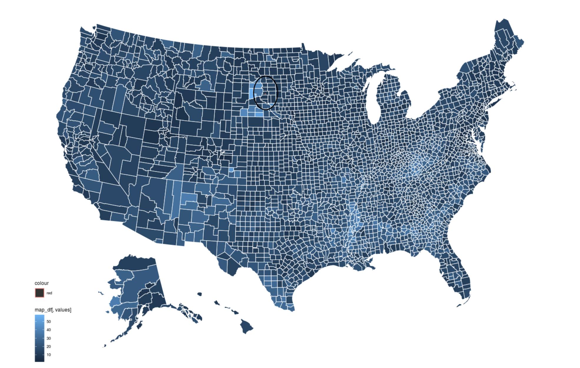
What I suspect is happening is that one layer (the original ggplot code) is projected using a different CRS system than the other layer -generated by plot_usmap. That second layer results in a very small red dot (see circle in map below). Not sure how to re-project without geos/gdal installed. See the map below with the black circle highlighting where the red dot is.

Yarkand

Any chance to use the fastshp package that you were using last time? – Kilogrammeter

@Kilogrammeter unfortunately that ended up being problematic with mapping at the county level but I'm open to it in theory. – Yarkand

Can you provide shapefiles that you have? Othrewise, is it OK to use any shapefiles? – Kilogrammeter

Here is one I used in the previous SO post if that works www2.census.gov/geo/tiger/TIGER2017/COUNTY/… otherwise anyone I can access online is fine for me so long as it includes HI AK at county level. thanks! – Yarkand

OK. Let me try. – Kilogrammeter

I still have issues to read any shapefiles with read.shp(). I do not know why. this package by hrbrmstr has shapefiles that you are probably interested in. I created shapefiles for you. If you can, can you try to download them from my git? If you can read these files with read.shp(), you will have good chance to draw the map you want, I think. – Kilogrammeter

A question. Do we need to use xzfile when we read shp files with read.shp? – Kilogrammeter

@Kilogrammeter preferably a zipped file bc shape files are a collection of various files and since I need access from the net it seems like a zipped shapefile is the way to go but I'm open to any solution that works, thanks! – Yarkand

@Kilogrammeter unfortunately hrbmstr's workflow relies on sf package, which requires units (similar to rgeos and rgdal needs non R libraries)..and unfortunately installing the package from hrbmstr also crashed my R environment... – Yarkand

I added all files in a folder and created a zip file, which stays at my git. The same page above. Can you get it and see if you can use that with fastshp? Since census data is also just shapefile, there should not be any difference, right? Or is there any? – Kilogrammeter

@Kilogrammeter I was unable to unzip from the command line in R. But at any rate, I'm more interested in the logic than which shapefile is used. When using fastshp with other Shapefiles I haven't been able to map county level boundaries properly (despite proper ordering and specification). – Yarkand

Since I cannot see what's happening on your side, I cannot do much. But if you can successfully import county-level shapefiles, you want to see what kind of information you have. Can you find parts? That was the column indicating index for each polygon. Presumably, there should be an index number for each county. If you can identify such information, you need to create group variable for each county in each state as I was doing for you last time. In case you cannot import any county-level polygon data in R, I think you want to contact the package author. – Kilogrammeter

As far as I see, the package was written several years ago and the author have left it. But it is worth sending a message and seek some help. – Kilogrammeter

does it have to be a static map? – Sagunto

If you have geojson, then library(geojsonsf) can read it and convert it to sf, without a dependency on sf – Sagunto

@Sagunto yes, no plotly please, I'll take a look at geojsonsf, thanks! – Yarkand

@Sagunto unfortunately it seems that to plot an sf object one needs access to the sf library (even if just using geom_sf in ggplot2) and sf depends on geos, which I cannot install. – Yarkand

ok. For what it's worth, library(mapdeck) can plot sf objects without depending on library(sf), BUT, it's an interactive map. – Sagunto

@SymbolixAU, thank you. Although, that won't help for my current needs, its very good to know! And thanks for your contribution to the R community with that package! Looks promising, I'll def check it out! – Yarkand

Answer 1

Ok after some suggestions from the package author and some of my own tinkering around I was finally able to get my desired output.

This approach is ideal for folks looking to generate a US map w/ Alaska and Hawaii included who...

1) Do not have the ability to install non-R packages in the environment their R engine is running on (e.g. lack admin access)

2) Need to map both county and state boundaries using contrasting colors

library(dplyr)
library(ggplot2)
library(usmap)

#Example data (poverty rates)
county_data<-read.csv("https://www.ers.usda.gov/webdocs/DataFiles/48747/PovertyEstimates.csv?v=2529") %>% #
  filter(Area_name != "United States") %>%
  select(FIPStxt, Stabr, Area_name, PCTPOVALL_2018) %>%
  rename(fips = FIPStxt)

states <- plot_usmap("states", 
                     color = "red",
                     fill = alpha(0.01)) #this parameter is necessary to get counties to show on top of states
counties <- plot_usmap(data = county_data, 
                       values = "PCTPOVALL_2018",
                       color = "black",
                       size = 0.1)

Using the layers meta info already embedded in the data from us_map

ggplot() +
  counties$layers[[1]] + #counties needs to be on top of states for this to work
  states$layers[[1]] +
  counties$theme + 
  coord_equal() +
  theme(legend.position="none") +
  scale_fill_gradient(low='white', high='grey20') #toggle fill schema using vanilla ggplot scale_fill function

Using just the raw data obtained from the us_map package

ggplot() +  
  geom_polygon(data=counties[[1]], 
               aes(x=x, 
                   y=y, 
                   group=group, 
                   fill = counties[[1]]$PCTPOVALL_2018), 
               color = "black",
               size = 0.1) +  
  geom_polygon(data=states[[1]], 
               aes(x=x, 
                   y=y, 
                   group=group), 
               color = "red", 
               fill = alpha(0.01)) + 
  coord_equal() +
  theme_map() +
  theme(legend.position="none") +
  scale_fill_gradient(low='white', high='grey20')

Yarkand

Using the layers meta-info method, I get Error in FUN(X[[i]], ...) : object 'x' not found. In fact, any variation of ggplot() + usmap$layers raises the same error. Any idea what's going on? – Pleven

I would have to see your code to troubleshoot. If you follow the exact steps from above you should be able to replicate. – Yarkand

I copy pasted your code to make sure, but it gives me the same error. Simplest code to reproduce the error: ggplot() + plot_usmap()$layers[[1]]. I'm using ggplot2_3.3.2 and usmap_0.5.1, in case that matters. – Pleven

Ofc, it isn't. But your code doesn't work either. I was just showing the easiest way to reproduce the error. Just to be clear, your second version (Using just the raw data obtained from the us_map package) works. The first one doesn't. – Pleven

For anybody else with the same problem, it seems that usmap 0.5.0 broke this functionality. A bug fix is in the works. Meanwhile, use an earlier version to get this to work. – Pleven