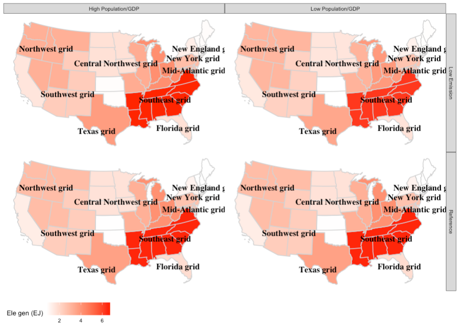
How merge specific states together by group with one label in ggplot2 in R?

Asked 22/6, 2022 at 0:10 Answered 22/6, 2022 at 7:12

I want to plot Electric grid map for U.S. So I need to merge specific states together . I want to plot border for those state together but it not working. Also just one label per each group. This is my data : [https://iastate.box.com/s/12xru62lvmbbkrohsn7b4wwexq11umn7] This is my code:

# Join and arrange
 states <- us_map(exclude = c("AK", "HI"))
 states_data <- left_join(states, myinput, by = c("abbr" = "region")) |> 
 arrange(emission, growth, group, order)

ggplot(states_data, aes(x, y, fill = value, group = group, subgroup = grid)) +
geom_polygon()+
scale_fill_continuous(low = "white", high = "red", name = "Ele gen (EJ)", label = 
scales::comma) +
facet_grid(emission~growth) +
coord_equal() +
ggthemes::theme_map() +
theme(legend.position = "bottom")+
geom_text(aes(x, y, label = grid),size = 5,family = "serif",
        data = states_data, vjust = 1.2, nudge_y = -100000,check_overlap = T)+
geom_polygon(aes(color = "Border", group=grid),fill = NA,color = "black")

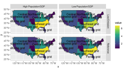
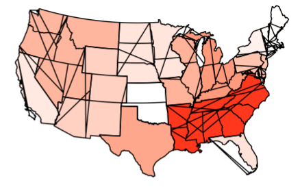
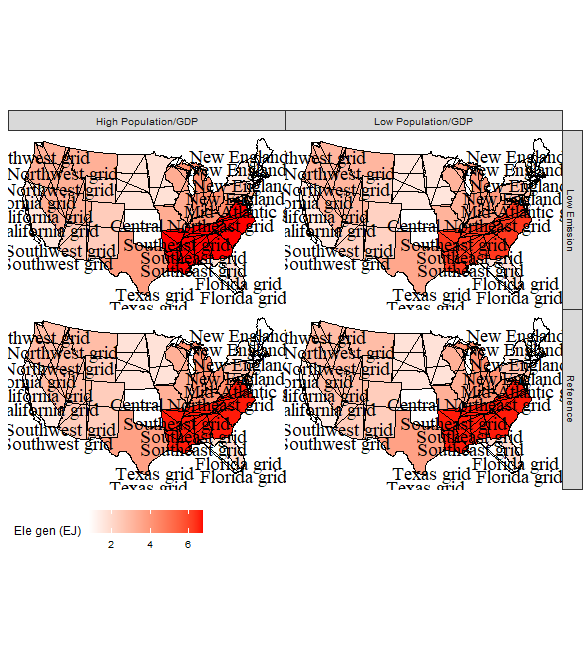
And this the output which is not what I have in my mid:

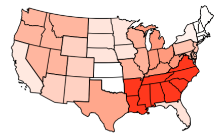
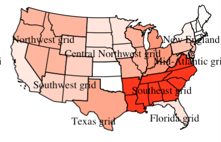
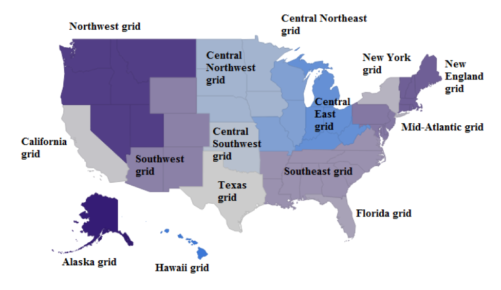
I want to plot these regions (plus borders to specify because I can't show them with different color)

data

structure(list(region = c("AL", "AR", "AZ", "CA", "CO", "CT", 
"DC", "DE", "FL", "GA", "IA", "ID", "IL", "IN", "KS", "KY", "LA", 
"MA", "MD", "ME", "MI", "MN", "MO", "MS", "MT", "NC", "ND", "NE", 
"NH", "NJ", "NM", "NV", "NY", "OH", "OK", "OR", "PA", "RI", "SC", 
"SD", "TN", "TX", "UT", "VA", "VT", "WA", "WI", "WV", "WY", "AL", 
"AR", "AZ", "CA", "CO", "CT", "DC", "DE", "FL", "GA", "IA", "ID", 
"IL", "IN", "KS", "KY", "LA", "MA", "MD", "ME", "MI", "MN", "MO", 
"MS", "MT", "NC", "ND", "NE", "NH", "NJ", "NM", "NV", "NY", "OH", 
"OK", "OR", "PA", "RI", "SC", "SD", "TN", "TX", "UT", "VA", "VT", 
"WA", "WI", "WV", "WY", "AL", "AR", "AZ", "CA", "CO", "CT", "DC", 
"DE", "FL", "GA", "IA", "ID", "IL", "IN", "KS", "KY", "LA", "MA", 
"MD", "ME", "MI", "MN", "MO", "MS", "MT", "NC", "ND", "NE", "NH", 
"NJ", "NM", "NV", "NY", "OH", "OK", "OR", "PA", "RI", "SC", "SD", 
"TN", "TX", "UT", "VA", "VT", "WA", "WI", "WV", "WY", "AL", "AR", 
"AZ", "CA", "CO", "CT", "DC", "DE", "FL", "GA", "IA", "ID", "IL", 
"IN", "KS", "KY", "LA", "MA", "MD", "ME", "MI", "MN", "MO", "MS", 
"MT", "NC", "ND", "NE", "NH", "NJ", "NM", "NV", "NY", "OH", "OK", 
"OR", "PA", "RI", "SC", "SD", "TN", "TX", "UT", "VA", "VT", "WA", 
"WI", "WV", "WY"), value = c(6.22256321333333, 6.22256321333333, 
2.20794523906666, 1.49034165333333, 2.20794523906666, 0.826546816817333, 
2.61905459786667, 2.61905459786667, 1.65110329, 6.22256321333333, 
1.59528739166667, 3.0363665376, 3.13763399333332, 3.865420576, 
0.790624669333333, 3.865420576, 6.22256321333333, 0.826546816817333, 
2.61905459786667, 0.826546816817333, 3.865420576, 1.59528739166667, 
3.13763399333332, 6.22256321333333, 3.0363665376, 6.22256321333333, 
1.59528739166667, 1.59528739166667, 0.826546816817333, 2.61905459786667, 
2.20794523906666, 3.0363665376, 1.21040939333333, 3.865420576, 
0.790624669333333, 3.0363665376, 2.61905459786667, 0.826546816817333, 
6.22256321333333, 1.59528739166667, 6.22256321333333, 3.50149982333333, 
3.0363665376, 6.22256321333333, 0.826546816817333, 3.0363665376, 
3.13763399333332, 3.865420576, 2.20794523906666, 6.58823506033333, 
6.58823506033333, 2.33729970666667, 1.35043392, 2.33729970666667, 
0.7918773089276, 2.64941819863333, 2.64941819863333, 1.84968858666667, 
6.58823506033333, 1.69423596966667, 2.82831107136667, 3.22375391666666, 
4.14114214399999, 0.816646300333333, 4.14114214399999, 6.58823506033333, 
0.7918773089276, 2.64941819863333, 0.7918773089276, 4.14114214399999, 
1.69423596966667, 3.22375391666666, 6.58823506033333, 2.82831107136667, 
6.58823506033333, 1.69423596966667, 1.69423596966667, 0.7918773089276, 
2.64941819863333, 2.33729970666667, 2.82831107136667, 1.15469864333333, 
4.14114214399999, 0.816646300333333, 2.82831107136667, 2.64941819863333, 
0.7918773089276, 6.58823506033333, 1.69423596966667, 6.58823506033333, 
3.66557223, 2.82831107136667, 6.58823506033333, 0.7918773089276, 
2.82831107136667, 3.22375391666666, 4.14114214399999, 2.33729970666667, 
6.72966092166666, 6.72966092166666, 2.3737108016, 1.58503659, 
2.3737108016, 0.884016546345666, 2.8041352651, 2.8041352651, 
1.73653393333333, 6.72966092166666, 1.73917558366667, 3.23410557176666, 
3.34795298333333, 4.19485727566666, 0.859289106, 4.19485727566666, 
6.72966092166666, 0.884016546345666, 2.8041352651, 0.884016546345666, 
4.19485727566666, 1.73917558366667, 3.34795298333333, 6.72966092166666, 
3.23410557176666, 6.72966092166666, 1.73917558366667, 1.73917558366667, 
0.884016546345666, 2.8041352651, 2.3737108016, 3.23410557176666, 
1.28265139333333, 4.19485727566666, 0.859289106, 3.23410557176666, 
2.8041352651, 0.884016546345666, 6.72966092166666, 1.73917558366667, 
6.72966092166666, 3.79724887666667, 3.23410557176666, 6.72966092166666, 
0.884016546345666, 3.23410557176666, 3.34795298333333, 4.19485727566666, 
2.3737108016, 6.58823506033333, 6.58823506033333, 2.33729970666667, 
1.35043392, 2.33729970666667, 0.7918773089276, 2.64941819863333, 
2.64941819863333, 1.84968858666667, 6.58823506033333, 1.69423596966667, 
2.82831107136667, 3.22375391666666, 4.14114214399999, 0.816646300333333, 
4.14114214399999, 6.58823506033333, 0.7918773089276, 2.64941819863333, 
0.7918773089276, 4.14114214399999, 1.69423596966667, 3.22375391666666, 
6.58823506033333, 2.82831107136667, 6.58823506033333, 1.69423596966667, 
1.69423596966667, 0.7918773089276, 2.64941819863333, 2.33729970666667, 
2.82831107136667, 1.15469864333333, 4.14114214399999, 0.816646300333333, 
2.82831107136667, 2.64941819863333, 0.7918773089276, 6.58823506033333, 
1.69423596966667, 6.58823506033333, 3.66557223, 2.82831107136667, 
6.58823506033333, 0.7918773089276, 2.82831107136667, 3.22375391666666, 
4.14114214399999, 2.33729970666667), grid = c("Southeast grid", 
"Southeast grid", "Southwest grid", "California grid", "Southwest grid", 
"New England grid", "Mid-Atlantic grid", "Mid-Atlantic grid", 
"Florida grid", "Southeast grid", "Central Northwest grid", "Northwest grid", 
"Central Northeast grid", "Central East grid", "Central Southwest grid", 
"Central East grid", "Southeast grid", "New England grid", "Mid-Atlantic grid", 
"New England grid", "Central East grid", "Central Northwest grid", 
"Central Northeast grid", "Southeast grid", "Northwest grid", 
"Southeast grid", "Central Northwest grid", "Central Northwest grid", 
"New England grid", "Mid-Atlantic grid", "Southwest grid", "Northwest grid", 
"New York grid", "Central East grid", "Central Southwest grid", 
"Northwest grid", "Mid-Atlantic grid", "New England grid", "Southeast grid", 
"Central Northwest grid", "Southeast grid", "Texas grid", "Northwest grid", 
"Southeast grid", "New England grid", "Northwest grid", "Central Northeast grid", 
"Central East grid", "Southwest grid", "Southeast grid", "Southeast grid", 
"Southwest grid", "California grid", "Southwest grid", "New England grid", 
"Mid-Atlantic grid", "Mid-Atlantic grid", "Florida grid", "Southeast grid", 
"Central Northwest grid", "Northwest grid", "Central Northeast grid", 
"Central East grid", "Central Southwest grid", "Central East grid", 
"Southeast grid", "New England grid", "Mid-Atlantic grid", "New England grid", 
"Central East grid", "Central Northwest grid", "Central Northeast grid", 
"Southeast grid", "Northwest grid", "Southeast grid", "Central Northwest grid", 
"Central Northwest grid", "New England grid", "Mid-Atlantic grid", 
"Southwest grid", "Northwest grid", "New York grid", "Central East grid", 
"Central Southwest grid", "Northwest grid", "Mid-Atlantic grid", 
"New England grid", "Southeast grid", "Central Northwest grid", 
"Southeast grid", "Texas grid", "Northwest grid", "Southeast grid", 
"New England grid", "Northwest grid", "Central Northeast grid", 
"Central East grid", "Southwest grid", "Southeast grid", "Southeast grid", 
"Southwest grid", "California grid", "Southwest grid", "New England grid", 
"Mid-Atlantic grid", "Mid-Atlantic grid", "Florida grid", "Southeast grid", 
"Central Northwest grid", "Northwest grid", "Central Northeast grid", 
"Central East grid", "Central Southwest grid", "Central East grid", 
"Southeast grid", "New England grid", "Mid-Atlantic grid", "New England grid", 
"Central East grid", "Central Northwest grid", "Central Northeast grid", 
"Southeast grid", "Northwest grid", "Southeast grid", "Central Northwest grid", 
"Central Northwest grid", "New England grid", "Mid-Atlantic grid", 
"Southwest grid", "Northwest grid", "New York grid", "Central East grid", 
"Central Southwest grid", "Northwest grid", "Mid-Atlantic grid", 
"New England grid", "Southeast grid", "Central Northwest grid", 
"Southeast grid", "Texas grid", "Northwest grid", "Southeast grid", 
"New England grid", "Northwest grid", "Central Northeast grid", 
"Central East grid", "Southwest grid", "Southeast grid", "Southeast grid", 
"Southwest grid", "California grid", "Southwest grid", "New England grid", 
"Mid-Atlantic grid", "Mid-Atlantic grid", "Florida grid", "Southeast grid", 
"Central Northwest grid", "Northwest grid", "Central Northeast grid", 
"Central East grid", "Central Southwest grid", "Central East grid", 
"Southeast grid", "New England grid", "Mid-Atlantic grid", "New England grid", 
"Central East grid", "Central Northwest grid", "Central Northeast grid", 
"Southeast grid", "Northwest grid", "Southeast grid", "Central Northwest grid", 
"Central Northwest grid", "New England grid", "Mid-Atlantic grid", 
"Southwest grid", "Northwest grid", "New York grid", "Central East grid", 
"Central Southwest grid", "Northwest grid", "Mid-Atlantic grid", 
"New England grid", "Southeast grid", "Central Northwest grid", 
"Southeast grid", "Texas grid", "Northwest grid", "Southeast grid", 
"New England grid", "Northwest grid", "Central Northeast grid", 
"Central East grid", "Southwest grid"), emission = c("Low Emission", 
"Low Emission", "Low Emission", "Low Emission", "Low Emission", 
"Low Emission", "Low Emission", "Low Emission", "Low Emission", 
"Low Emission", "Low Emission", "Low Emission", "Low Emission", 
"Low Emission", "Low Emission", "Low Emission", "Low Emission", 
"Low Emission", "Low Emission", "Low Emission", "Low Emission", 
"Low Emission", "Low Emission", "Low Emission", "Low Emission", 
"Low Emission", "Low Emission", "Low Emission", "Low Emission", 
"Low Emission", "Low Emission", "Low Emission", "Low Emission", 
"Low Emission", "Low Emission", "Low Emission", "Low Emission", 
"Low Emission", "Low Emission", "Low Emission", "Low Emission", 
"Low Emission", "Low Emission", "Low Emission", "Low Emission", 
"Low Emission", "Low Emission", "Low Emission", "Low Emission", 
"Reference", "Reference", "Reference", "Reference", "Reference", 
"Reference", "Reference", "Reference", "Reference", "Reference", 
"Reference", "Reference", "Reference", "Reference", "Reference", 
"Reference", "Reference", "Reference", "Reference", "Reference", 
"Reference", "Reference", "Reference", "Reference", "Reference", 
"Reference", "Reference", "Reference", "Reference", "Reference", 
"Reference", "Reference", "Reference", "Reference", "Reference", 
"Reference", "Reference", "Reference", "Reference", "Reference", 
"Reference", "Reference", "Reference", "Reference", "Reference", 
"Reference", "Reference", "Reference", "Reference", "Low Emission", 
"Low Emission", "Low Emission", "Low Emission", "Low Emission", 
"Low Emission", "Low Emission", "Low Emission", "Low Emission", 
"Low Emission", "Low Emission", "Low Emission", "Low Emission", 
"Low Emission", "Low Emission", "Low Emission", "Low Emission", 
"Low Emission", "Low Emission", "Low Emission", "Low Emission", 
"Low Emission", "Low Emission", "Low Emission", "Low Emission", 
"Low Emission", "Low Emission", "Low Emission", "Low Emission", 
"Low Emission", "Low Emission", "Low Emission", "Low Emission", 
"Low Emission", "Low Emission", "Low Emission", "Low Emission", 
"Low Emission", "Low Emission", "Low Emission", "Low Emission", 
"Low Emission", "Low Emission", "Low Emission", "Low Emission", 
"Low Emission", "Low Emission", "Low Emission", "Low Emission", 
"Reference", "Reference", "Reference", "Reference", "Reference", 
"Reference", "Reference", "Reference", "Reference", "Reference", 
"Reference", "Reference", "Reference", "Reference", "Reference", 
"Reference", "Reference", "Reference", "Reference", "Reference", 
"Reference", "Reference", "Reference", "Reference", "Reference", 
"Reference", "Reference", "Reference", "Reference", "Reference", 
"Reference", "Reference", "Reference", "Reference", "Reference", 
"Reference", "Reference", "Reference", "Reference", "Reference", 
"Reference", "Reference", "Reference", "Reference", "Reference", 
"Reference", "Reference", "Reference", "Reference"), growth = c("Low Population/GDP", 
"Low Population/GDP", "Low Population/GDP", "Low Population/GDP", 
"Low Population/GDP", "Low Population/GDP", "Low Population/GDP", 
"Low Population/GDP", "Low Population/GDP", "Low Population/GDP", 
"Low Population/GDP", "Low Population/GDP", "Low Population/GDP", 
"Low Population/GDP", "Low Population/GDP", "Low Population/GDP", 
"Low Population/GDP", "Low Population/GDP", "Low Population/GDP", 
"Low Population/GDP", "Low Population/GDP", "Low Population/GDP", 
"Low Population/GDP", "Low Population/GDP", "Low Population/GDP", 
"Low Population/GDP", "Low Population/GDP", "Low Population/GDP", 
"Low Population/GDP", "Low Population/GDP", "Low Population/GDP", 
"Low Population/GDP", "Low Population/GDP", "Low Population/GDP", 
"Low Population/GDP", "Low Population/GDP", "Low Population/GDP", 
"Low Population/GDP", "Low Population/GDP", "Low Population/GDP", 
"Low Population/GDP", "Low Population/GDP", "Low Population/GDP", 
"Low Population/GDP", "Low Population/GDP", "Low Population/GDP", 
"Low Population/GDP", "Low Population/GDP", "Low Population/GDP", 
"Low Population/GDP", "Low Population/GDP", "Low Population/GDP", 
"Low Population/GDP", "Low Population/GDP", "Low Population/GDP", 
"Low Population/GDP", "Low Population/GDP", "Low Population/GDP", 
"Low Population/GDP", "Low Population/GDP", "Low Population/GDP", 
"Low Population/GDP", "Low Population/GDP", "Low Population/GDP", 
"Low Population/GDP", "Low Population/GDP", "Low Population/GDP", 
"Low Population/GDP", "Low Population/GDP", "Low Population/GDP", 
"Low Population/GDP", "Low Population/GDP", "Low Population/GDP", 
"Low Population/GDP", "Low Population/GDP", "Low Population/GDP", 
"Low Population/GDP", "Low Population/GDP", "Low Population/GDP", 
"Low Population/GDP", "Low Population/GDP", "Low Population/GDP", 
"Low Population/GDP", "Low Population/GDP", "Low Population/GDP", 
"Low Population/GDP", "Low Population/GDP", "Low Population/GDP", 
"Low Population/GDP", "Low Population/GDP", "Low Population/GDP", 
"Low Population/GDP", "Low Population/GDP", "Low Population/GDP", 
"Low Population/GDP", "Low Population/GDP", "Low Population/GDP", 
"Low Population/GDP", "High Population/GDP", "High Population/GDP", 
"High Population/GDP", "High Population/GDP", "High Population/GDP", 
"High Population/GDP", "High Population/GDP", "High Population/GDP", 
"High Population/GDP", "High Population/GDP", "High Population/GDP", 
"High Population/GDP", "High Population/GDP", "High Population/GDP", 
"High Population/GDP", "High Population/GDP", "High Population/GDP", 
"High Population/GDP", "High Population/GDP", "High Population/GDP", 
"High Population/GDP", "High Population/GDP", "High Population/GDP", 
"High Population/GDP", "High Population/GDP", "High Population/GDP", 
"High Population/GDP", "High Population/GDP", "High Population/GDP", 
"High Population/GDP", "High Population/GDP", "High Population/GDP", 
"High Population/GDP", "High Population/GDP", "High Population/GDP", 
"High Population/GDP", "High Population/GDP", "High Population/GDP", 
"High Population/GDP", "High Population/GDP", "High Population/GDP", 
"High Population/GDP", "High Population/GDP", "High Population/GDP", 
"High Population/GDP", "High Population/GDP", "High Population/GDP", 
"High Population/GDP", "High Population/GDP", "High Population/GDP", 
"High Population/GDP", "High Population/GDP", "High Population/GDP", 
"High Population/GDP", "High Population/GDP", "High Population/GDP", 
"High Population/GDP", "High Population/GDP", "High Population/GDP", 
"High Population/GDP", "High Population/GDP", "High Population/GDP", 
"High Population/GDP", "High Population/GDP", "High Population/GDP", 
"High Population/GDP", "High Population/GDP", "High Population/GDP", 
"High Population/GDP", "High Population/GDP", "High Population/GDP", 
"High Population/GDP", "High Population/GDP", "High Population/GDP", 
"High Population/GDP", "High Population/GDP", "High Population/GDP", 
"High Population/GDP", "High Population/GDP", "High Population/GDP", 
"High Population/GDP", "High Population/GDP", "High Population/GDP", 
"High Population/GDP", "High Population/GDP", "High Population/GDP", 
"High Population/GDP", "High Population/GDP", "High Population/GDP", 
"High Population/GDP", "High Population/GDP", "High Population/GDP", 
"High Population/GDP", "High Population/GDP", "High Population/GDP", 
"High Population/GDP", "High Population/GDP", "High Population/GDP"
)), class = c("tbl_df", "tbl", "data.frame"), row.names = c(NA, 
-196L))

Marthamarthe answered 22/6, 2022 at 0:10 Comment(1)

related #9441936 – Kata 22/6, 2022 at 6:51

You will need to use shapefiles/ simple feature [sf] objects rather than mere data frames.

The usmap package is a high level package which is meant for convenient production of standard US maps. It does not come with shapefiles but contains the polygon data in actual data frames (provided by the package usmapdata. Custom merging of states is not facilitated by this package.

Merging polygons in a data frame is not impossible, but it's not easy. It would also be re-inventing the wheel, as the sf package was built just for things like this. But it works only with shapefiles / sf objects.

Good news, the US is not an unpopular country in the R world, and there are other R packages which contain US map data, e.g. USAboundaries, which comes with shapefiles.

The sf package allows you to merge (here this process is called unionise) polygons easily, e.g. with simple summarising. (see below).

You can then use ggplot2's very own geom_sf for the unionised polygons and geom_sf_text or geom_sf_label for the labels.

Further comments in the code.

library(tidyverse)
## use for example this for US shapefile maps
library(USAboundaries)
## you will need the sf package for some stuff
library(sf)

# my_data <- ... from your question above

states <- us_states()
states <- states[!states$name %in% c("Alaska", "Hawaii"),]
##remove arrange
states_data <- left_join(states, my_data, by = c("state_abbr" = "region" )) %>%
## there is an NA value that needs removal
drop_na(grid)

## this is to unionise the polygons
custom_grids <- 
  states_data %>%
## group by all the variables that occur in the facets
  group_by(grid, emission, growth) %>%
  summarise(value = mean(value))

## you can now plot the unionised polygon sf object with geom_sf and geom_sf_text for labels
ggplot(custom_grids) +
  geom_sf(aes(fill = value)) +
  geom_sf_text(aes(label = grid), check_overlap = T)+
  scale_fill_viridis_c() +
  facet_grid(emission~growth)

Kata answered 22/6, 2022 at 7:12 Comment(6)

Thanks, but I want border for Grids not states! I want to show grid with borders. – Marthamarthe 22/6, 2022 at 16:27

Also one of the grid's name is missing on the plot you shared! – Marthamarthe 22/6, 2022 at 16:34

@Marthamarthe which grid is that? – Kata 22/6, 2022 at 16:53

Electric grid, which you labeled on the map. For example the Central Southwest grid includes 'Ks' and 'OK' states. – Marthamarthe 22/6, 2022 at 18:31

You can see that some state are in same color because their values are same (they are in a same grid) because the values are based on the grids. I want to merge states with column 'grid'. – Marthamarthe 22/6, 2022 at 18:37

@Marthamarthe please see updated answer – Kata 23/6, 2022 at 12:31

I couldn't find an overly simple way of making this happen, but I can help you make it happen.

First, I calculated the median x and y for each of the groups and facets.

mm <- states_data %>% 
  group_by(growth, emission, grid) %>% 
  summarise(x = median(x), y = median(y))

Then I looked for the closest line row of data that matched these coordinates for placing the label. I created a function, a vector of NA (to be updated), and then went through each of the medians to find the corresponding row in the data (states_data). This creates another column for the data, but the grid strings are only in the rows that were identified as the quasi-center of each grid.

mdist <- function(mm, df1) { #vector mm contains medians; df1 contains points to compare
  x = mm$x
  y = mm$y
  df2 <- df1 %>% mutate(rn = 1:nrow(.)) %>% 
    filter(grid == mm$grid, growth == mm$growth, emission == mm$emission)
  df3 <- data.frame(V1 = sqrt((abs(df2$x) - abs(x))^2 + (abs(df2$y) - abs(y))^2),
                    rn = df2$rn,
                    grid = mm$grid) %>% 
    filter(V1 == min(V1))
  return(df3[1, ])
}

arr <- rep(NA, nrow(states_data))
invisible(
  map(1:nrow(mm),
      function(j) {
        gimme <- mdist(mm[j, ], states_data)
        arr[gimme$rn] <<- gimme$grid
      }))

Now, this column grid2 is used for the labels.

I noticed that you have group and subgroup in your call for ggplot. However, your subgroup has more divisions than group, that's what's causing the scribbling (for lack of a better word). This is what I mean:

I switched the group/subgroup calls in ggplot for this reason. (You may have wanted that, so I just wanted to explain what and why I did what I did.)

I also noticed that your grid is on top of the text and the same color, which sort of drowns out the words. You used nudge_y, but I think you might get a bit more bang with hjust, as well.

This is what I used:

ggplot(states_data, aes(x, y, fill = value, subgroup = group, group = grid)) +
  geom_polygon()+
  scale_fill_continuous(low = "white", high = "red", name = "Ele gen (EJ)", label = 
                          scales::comma) +
  facet_grid(emission~growth) +
  coord_equal() +
  ggthemes::theme_map() +
  theme(legend.position = "bottom") +
  geom_polygon(aes(color = "Border", group = grid),fill = NA, color = "lightgray") +
  geom_text(aes(label = grid2),size = 4, family = "serif", fontface = "bold",
            data = states_data, vjust = 1.2, hjust = .5, check_overlap = T)

It's not perfect. You're right-most labels are still running off the "page". However, this should get you going in the right direction.

Protege answered 22/6, 2022 at 5:50 Comment(3)

I am not sure that one needs to be so complicated (yet +1). Another option could be to combine the desired states to one "mega polygon" and then to use #9441936 (in particular the ggh4x package has a stat that calculates centroids). – Kata 22/6, 2022 at 6:52

Thanks, but I want border for Grids not states! I want to show grid with borders. Also some of the grid's name are missing on the plot you shared! – Marthamarthe 22/6, 2022 at 16:30

Every grid name in the column grid is on this map. If there is another grid name, please update your data in your question. In the meantime, I will try to work out the boundary regions you've requested. – Protege 23/6, 2022 at 2:58