Is there a way to remove the whitespace outside of a ggplot?

Question

I'm taking the code I use to create a static map to include on a shiny app. I have an issue though where the plot size is much larger than the actual plot, so the layout looks off. Is there any way to reduce this whitespace on the outside of the plot?

If possible I'd like the output to be only the plot itself.

# reprex
library(terra)
library(sf)
library(magrittr)
library(ggplot2)

lux <- vect(system.file("ex/lux.shp", package = "terra"))

p <- lux %>% 
  st_as_sf() %>%
  ggplot() +
  geom_sf(aes(fill = NAME_2), colour = "white", size = 0.2) +
  theme(legend.position = "None") +
# found online - removes the whitespace around the plot but not the external whitespace
  theme(plot.margin=grid::unit(c(0,0,0,0), "mm")) 

p

Bracteate

Answer 1

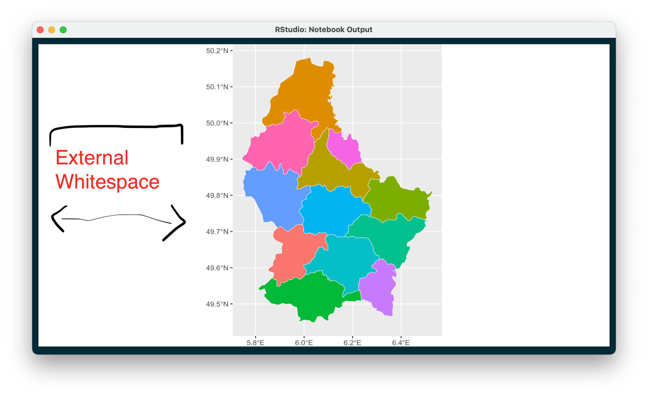
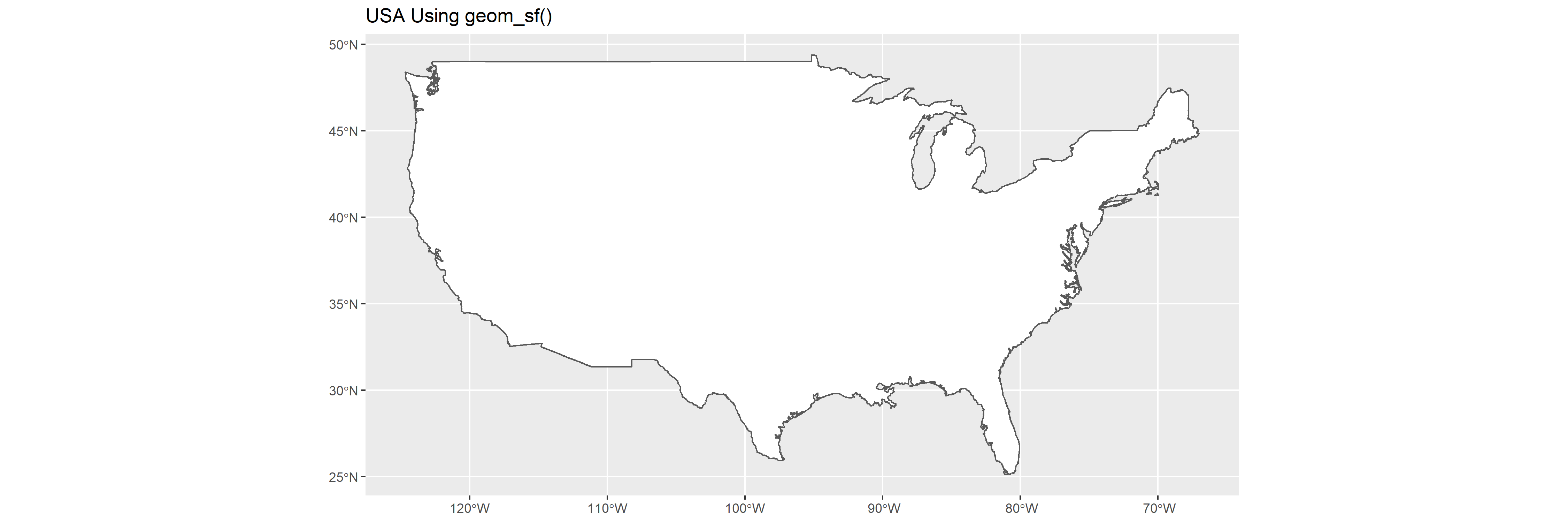
The reason your plot contains the whitespace is due to the constraints put on the coordinate system by geom_sf(). The aspect ratio of your plot normally adjusts itself to fit the size of the window in a typical plot, but in the case of a shapefile (sf), the aspect ratio is determined by the particular coordinate reference system, or CRS associated with that particular projection. You've seen this before in maps, where there is a distortion in each of the maps that happens due to trying to project the surface of a globe onto a 2D flat plane.

So, geom_sf() results in a map with the proper aspect ratio. If your view window or output image does not match that aspect ratio, then you will have whitespace at the sides or top to compensate. The way to solve the problem, then, is to either change the aspect ratio of your plot (which will not look right and is not a good idea) or have your output image or window match the aspect ratio of your plot.

TL;DR - use tmaptools::get_asp_ratio() to grab the aspect ratio of your plot object, then save the plot image with that aspect ratio.

Now for some explanatory images and such that help illustrate why geom_sf() functions differently than geom_polygon(), and how you can fix the issue in a representative example.

Maps using geom_polygon()

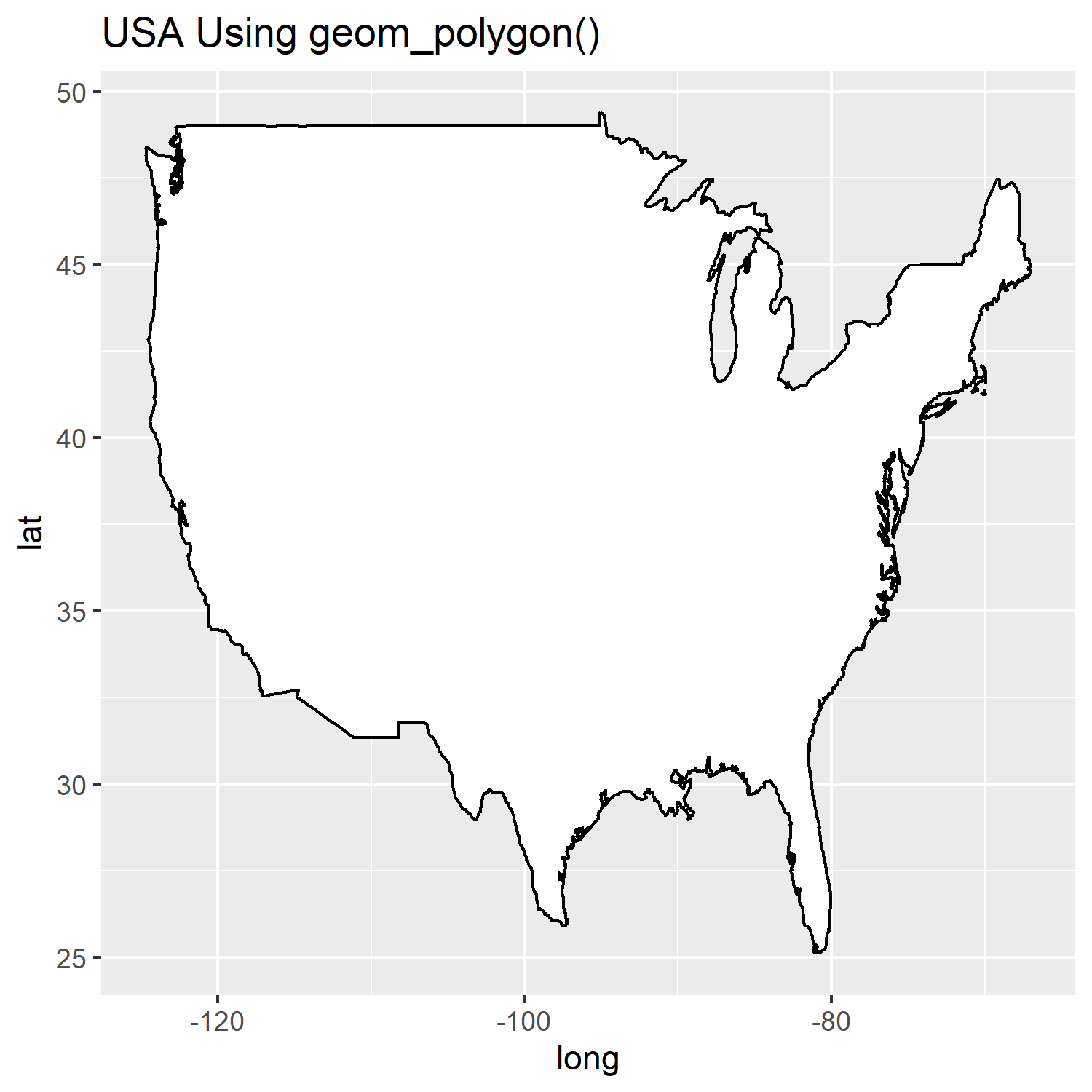
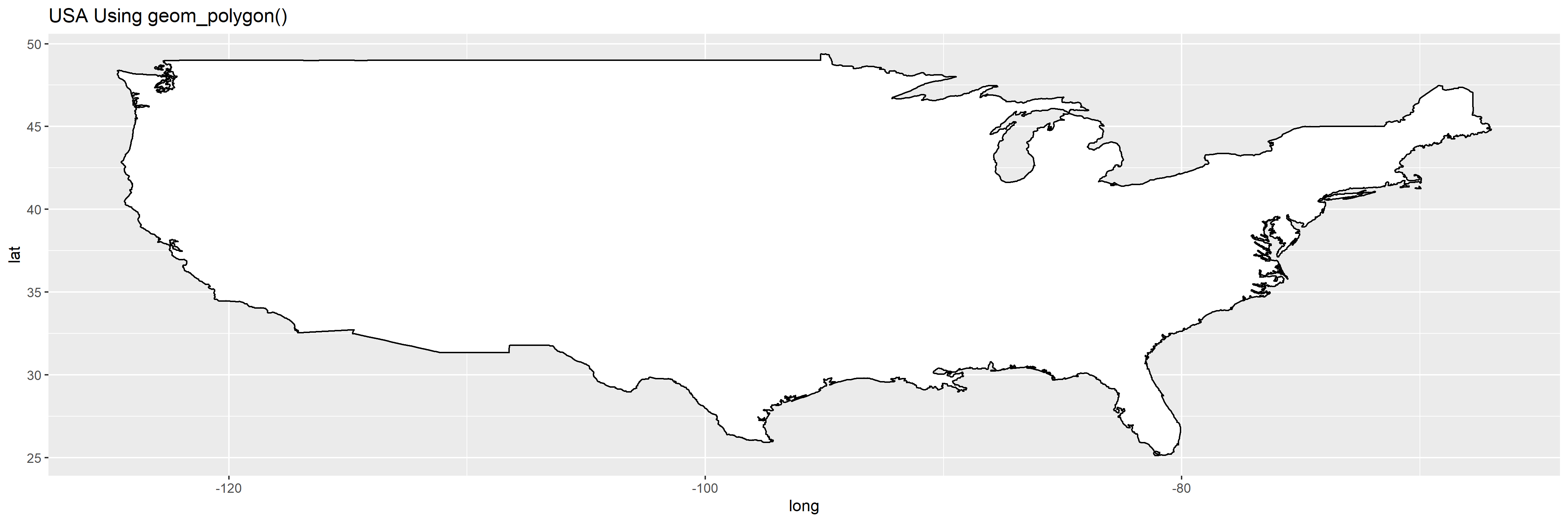
Unless you fix the ratio of the plot area with coord_fixed(), geom_polygon() will always squish and stretch as the output aspect ratio changes.

library(ggplot2)

my_map <- map_data("usa")
p1 <-
  ggplot(my_map, aes(long, lat)) +
  geom_polygon(aes(group=group), fill='white', color='black') +
  ggtitle('USA Using geom_polygon()')

Here's a square map:

ggsave('p1_square.png', plot=p1, width=5, height=5)

Here's a rectangle map:

ggsave('p1_rect.png', plot=p1, width=15, height=5)

Maps using geom_sf()

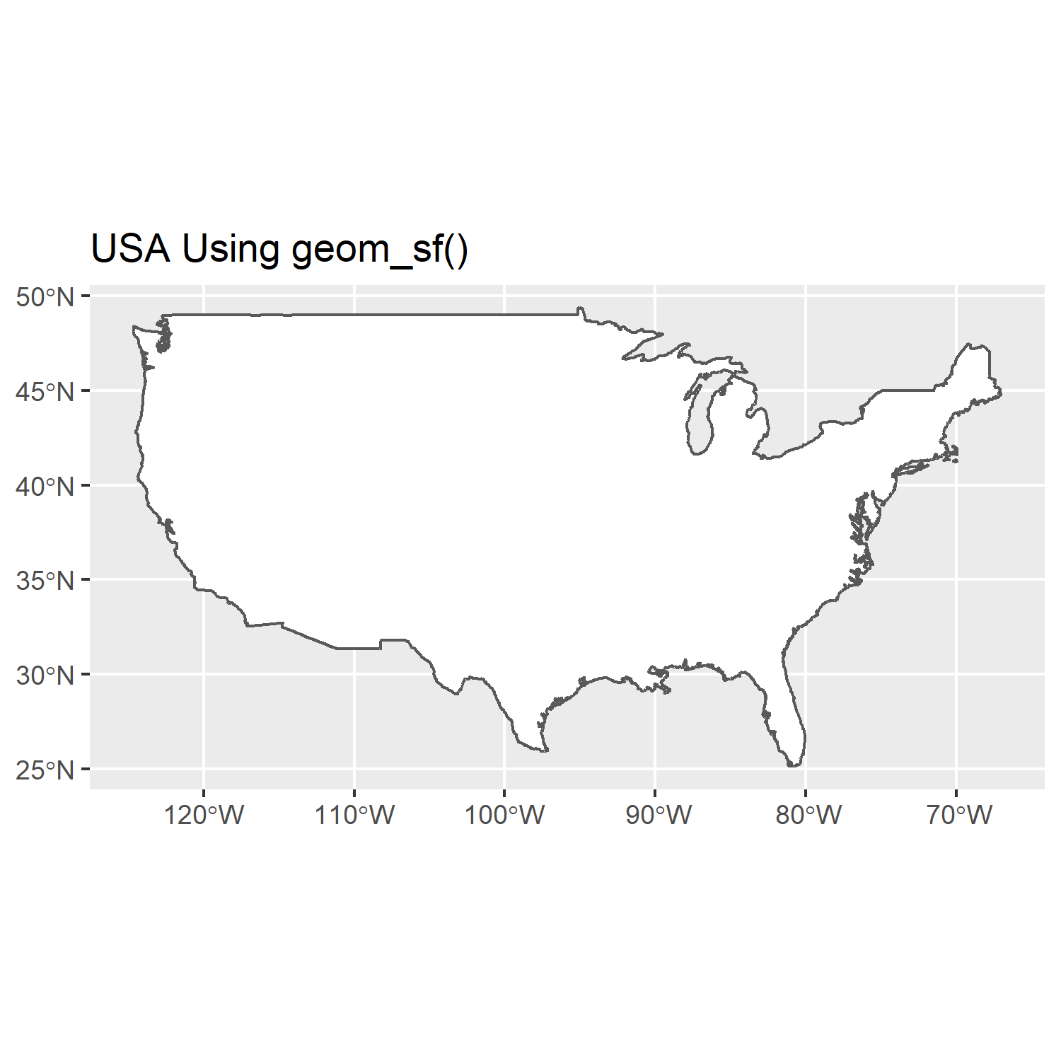
In comparison, you can see the maps with geom_sf() always maintain their aspect ratio, regardless of the size of the output.

library(sf)

world1 <- sf::st_as_sf(map('usa', plot = FALSE, fill = TRUE))
p2 <-
  ggplot() + geom_sf(data = world1, fill='white') + ggtitle('USA Using geom_sf()')

A square output:

ggsave('p2_square.png', plot=p2, width=5, height=5)

A rectangle output:

ggsave('p2_rect.png', plot=p2, width=15, height=5)

How to Remove Whitespace?

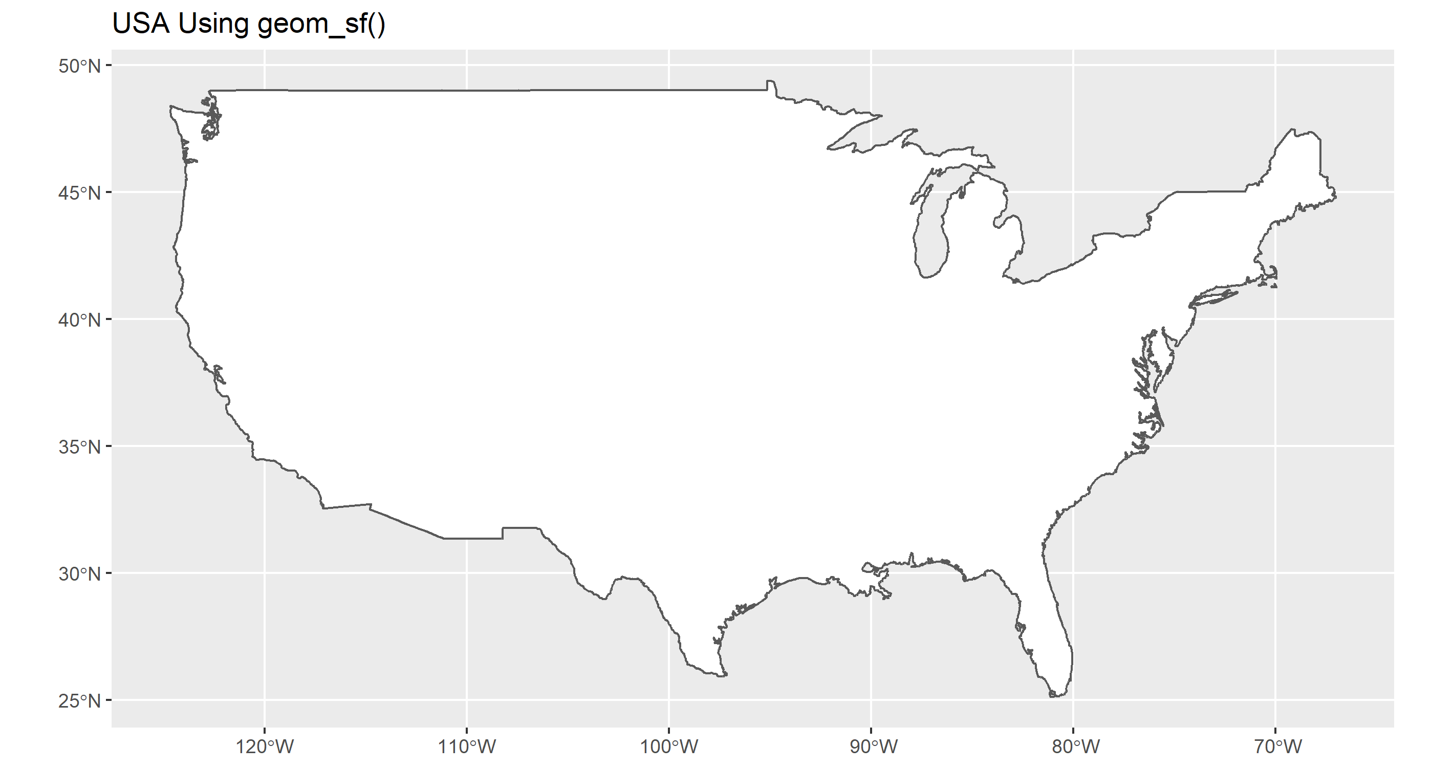
So, now it should be obvious why you have whitespace... but how do we remove it? Well, the answer is that you need to save your plot with the same aspect ratio given by the CRS used by your sf object. What you need is a way of getting that information. The function st_crs() in the sf package can get the name of the CRS used by your shapefile, but it doesn't outright give you the aspect ratio. For that, you can use the get_asp_ratio() function from the tmaptools library, then use that to calculate your width/height. It's important to note here that we need to use get_asp_ratio() on the sf object and not on the plot object. In this case, that's world1 and not p2.

plot_ratio <- get_asp_ratio(world1)
ggsave('p2_perfect.png', plot=p2, width = plot_ratio*5, height=5)

That gives us a plot output that perfectly matches the aspect ratio of your map:

Acceptant

Perfect! Thanks for the thorough explanation too – Bracteate