How to properly sample truncated distributions?

Question

I am trying to learn how to sample truncated distributions. To begin with I decided to try a simple example I found here example

I didn't really understand the division by the CDF, therefore I decided to tweak the algorithm a bit. Being sampled is an exponential distribution for values x>0 Here is an example python code:

# Sample exponential distribution for the case x>0
import numpy as np
import matplotlib.pyplot as plt
from scipy.stats import norm

def pdf(x):
        return x*np.exp(-x)

xvec=np.zeros(1000000)
x=1.
for i in range(1000000):
      a=x+np.random.normal()
      xs=x
      if a > 0. :
        xs=a
      A=pdf(xs)/pdf(x)
      if np.random.uniform()<A :
        x=xs
        xvec[i]=x

x=np.linspace(0,15,1000)
plt.plot(x,pdf(x))
plt.hist([x for x in xvec if x != 0],bins=150,normed=True)
plt.show()

Ant the output is:

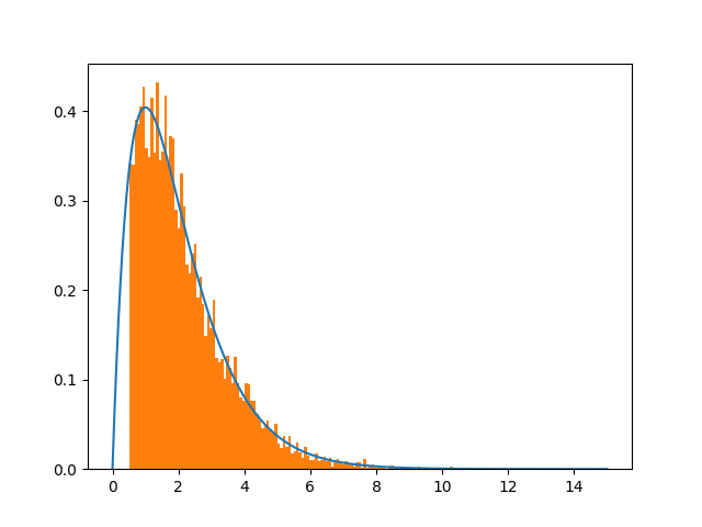
The code above seems to work fine only for when using the condition if a > 0. :, i.e. positive x, choosing another condition (e.g. if a > 0.5 :) produces wrong results.

Since my final goal was to sample a 2D-Gaussian - pdf on a truncated interval I tried extending the simple example using the exponential distribution (see the code below). Unfortunately, since the simple case didn't work, I assume that the code given below would yield wrong results.

I assume that all this can be done using the advanced tools of python. However, since my primary idea was to understand the principle behind, I would greatly appreciate your help to understand my mistake. Thank you for your help.

EDIT:

# code updated according to the answer of CrazyIvan 
from scipy.stats import multivariate_normal

RANGE=100000

a=2.06072E-02
b=1.10011E+00
a_range=[0.001,0.5]
b_range=[0.01, 2.5]
cov=[[3.1313994E-05,  1.8013737E-03],[ 1.8013737E-03,  1.0421529E-01]]

x=a
y=b
j=0

for i in range(RANGE):
    a_t,b_t=np.random.multivariate_normal([a,b],cov)
# accept if within bounds - all that is neded to truncate
    if a_range[0]<a_t and a_t<a_range[1] and b_range[0]<b_t and b_t<b_range[1]:
        print(dx,dy) 

EDIT:

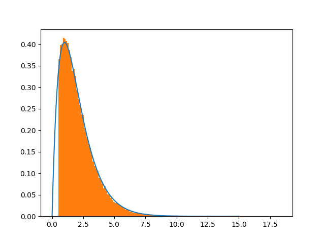
I changed the code by norming the analytic pdf according to this scheme, and according to the answers given by, @Crazy Ivan and @Leandro Caniglia , for the case where the bottom of the pdf is removed. That is dividing by (1-CDF(0.5)) since my accept condition is x>0.5. This seems again to show some discrepancies. Again the mystery prevails ..

import numpy as np
import matplotlib.pyplot as plt
from scipy.stats import norm

def pdf(x):
        return x*np.exp(-x)
# included the corresponding cdf
def cdf(x):
        return 1. -np.exp(-x)-x*np.exp(-x)

xvec=np.zeros(1000000)
x=1.
for i in range(1000000):
      a=x+np.random.normal()
      xs=x
      if a > 0.5 :
        xs=a
      A=pdf(xs)/pdf(x)
      if np.random.uniform()<A :
        x=xs
        xvec[i]=x

x=np.linspace(0,15,1000)
# new part norm the analytic pdf to fix the area
plt.plot(x,pdf(x)/(1.-cdf(0.5)))
plt.hist([x for x in xvec if x != 0],bins=200,normed=True)
plt.savefig("test_exp.png")
plt.show()

It seems that this can be cured by choosing larger shift size

shift=15.
a=x+np.random.normal()*shift.

which is in general an issue of the Metropolis - Hastings. See the graph below:

I also checked shift=150

Bottom line is that changing the shift size definitely improves the convergence. The misery is why, since the Gaussian is unbounded.

Binetta

Why do you say that the plot you get is wrong for a > 0.5? The excess area of the orange part seems to compensate the part below the curve with x<0.5, which is what you want so that the total orange area (i.e., the integral of the truncated pdf) equals 1. – Duck

Shouldn't I actually divide the ``pdf(x)` by the pdf(x)/(1-cdf(0.5)) at least this is the prescription for the case if the bottom of the distribution has been removed from the wiki article. en.wikipedia.org/wiki/Truncated_distribution. I included an example, but the sampling procedure seems to be biased still – Binetta

Yes, you should divide pdf(x)/(1-cdf(0.5)) in your case. This is precisely what my answer says (see below) because in your case B=1 and A=cdf(0.5). I've rewritten this part of the answer to make it clearer. – Duck

Actually the step size also matters. I tried to include some examples demonstrating this effect in my edit. – Binetta

thank you once again for the help. I get this, the problem is that I get values larger than the blue curve, corresponding to the 0.5<x<1.2 Of course to properly plot, I have to cut the unnecessary part from the blue curve. – Binetta

But that is ok. Discrepancies between "empirical" samples (which are random) and the theoretical curve decrease with the number of samples. In your case, with the number of steps. The curve depicts the theoretical behavior as the number of samples goes to infinity. – Duck

This problem prevails even at 1E8 iterations. – Binetta

Answer 1

You say you want to learn the basic idea of sampling a truncated distribution, but your source is a blog post about Metropolis–Hastings algorithm? Do you actually need this "method for obtaining a sequence of random samples from a probability distribution for which direct sampling is difficult"? Taking this as your starting point is like learning English by reading Shakespeare.

Truncated normal

For truncated normal, basic rejection sampling is all you need: generate samples for original distribution, reject those outside of bounds. As Leandro Caniglia noted, you should not expect truncated distribution to have the same PDF except on a shorter interval — this is plain impossible because the area under the graph of a PDF is always 1. If you cut off stuff from sides, there has to be more in the middle; the PDF gets rescaled.

It's quite inefficient to gather samples one by one, when you need 100000. I would grab 100000 normal samples at once, accept only those that fit; then repeat until I have enough. Example of sampling truncated normal between amin and amax:

import numpy as np
n_samples = 100000
amin, amax = -1, 2
samples = np.zeros((0,))    # empty for now
while samples.shape[0] < n_samples: 
    s = np.random.normal(0, 1, size=(n_samples,))
    accepted = s[(s >= amin) & (s <= amax)]
    samples = np.concatenate((samples, accepted), axis=0)
samples = samples[:n_samples]    # we probably got more than needed, so discard extra ones

And here is the comparison with the PDF curve, rescaled by division by cdf(amax) - cdf(amin) as explained above.

from scipy.stats import norm
_ = plt.hist(samples, bins=50, density=True)
t = np.linspace(-2, 3, 500)
plt.plot(t, norm.pdf(t)/(norm.cdf(amax) - norm.cdf(amin)), 'r')
plt.show()

Truncated multivariate normal

Now we want to keep the first coordinate between amin and amax, and the second between bmin and bmax. Same story, except there will be a 2-column array and the comparison with bounds is done in a relatively sneaky way:

(np.min(s - [amin, bmin], axis=1) >= 0) & (np.max(s - [amax, bmax], axis=1) <= 0)

This means: subtract amin, bmin from each row and keep only the rows where both results are nonnegative (meaning we had a >= amin and b >= bmin). Also do a similar thing with amax, bmax. Accept only the rows that meet both criteria.

n_samples = 10
amin, amax = -1, 2
bmin, bmax = 0.2, 2.4
mean = [0.3, 0.5]
cov = [[2, 1.1], [1.1, 2]]
samples = np.zeros((0, 2))   # 2 columns now
while samples.shape[0] < n_samples: 
    s = np.random.multivariate_normal(mean, cov, size=(n_samples,))
    accepted = s[(np.min(s - [amin, bmin], axis=1) >= 0) & (np.max(s - [amax, bmax], axis=1) <= 0)]
    samples = np.concatenate((samples, accepted), axis=0)
samples = samples[:n_samples, :]

Not going to plot, but here are some values: naturally, within bounds.

array([[ 0.43150033,  1.55775629],
       [ 0.62339265,  1.63506963],
       [-0.6723598 ,  1.58053835],
       [-0.53347361,  0.53513105],
       [ 1.70524439,  2.08226558],
       [ 0.37474842,  0.2512812 ],
       [-0.40986396,  0.58783193],
       [ 0.65967087,  0.59755193],
       [ 0.33383214,  2.37651975],
       [ 1.7513789 ,  1.24469918]])

Pinchpenny

Thank you very much for your answer. It seems to be much more simple, than what I was thinking. If I understand everything correctly a filter with an `if`` statement Is all I need. I have updated my code for the 2d truncated normal. Unfortunately I code all this in fortran, this is why I draw the samples one by one and accept and reject. Therefore, your elegant solution would be a bit difficult. – Binetta

Answer 2

To compute the truncated density function pdf_t from the entire density function pdf, do the following:

1. Let [a, b] be the truncation interval; (x axis)
2. Let A := cdf(a) and B := cdf(b); (cdf = non-truncated cumulative distribution function)
3. Then pdf_t(x) := pdf(x) / (B - A) if x in [a, b] and 0 elsewhere.

In cases where a = -infinity (resp. b = +infinity), take A := 0 (resp. B := 1).

---

As for the "mystery" you see

please note that your blue curve is wrong. It is not the pdf of your truncated distribution, it is just the pdf of the non-truncated one, scaled by the correct amount (division by 1-cdf(0.5)). The actual truncated pdf curve starts with a vertical line on x = 0.5 which goes up until it reaches your current blue curve. In other words, you only scaled the curve but forgot to truncate it, in this case to the left. Such a truncation corresponds to the "0 elsewhere" part of step 3 in the algorithm above.

Duck

Actually I was interested why I exceed the abscissa of the blue curve and why things improve if I increase the step size. Of course for the proper plot I have to delete the part of the blue curve, where no samples are drawn (corresponding to x<0.5) – Binetta

Answer 3

You can achieve this with inverse transform sampling.

It's quite easy using NumPy and SciPy:

import numpy as np
from scipy import stats


def truncated_normal_rvs(
    x_min: float,
    x_max: float,
    loc: float,
    scale: float,
    size: int,
) -> np.ndarray:
    quantile1 = stats.norm.cdf(x_min, loc=loc, scale=scale)
    quantile2 = stats.norm.cdf(x_max, loc=loc, scale=scale)

    return stats.norm.ppf(
        np.random.uniform(quantile1, quantile2, size=size),
        loc=loc,
        scale=scale,
    )

You can replace stats.norm with any other SciPy random variable. I ran into this myself when I needed a truncated chi-squared distribution, for which I used stats.chi2.

ppf is the "percent-point function", which takes a percentage (0.0 - 1.0) and returns a value Q for which P(x < Q) equals the given value (that is, it returns the corresponding percentile). It's the inverse of cdf.

You can sample a random variable by sampling (0.0, 1.0) uniformly and transforming the values with ppf (I believe that's how SciPy and NumPy do it). You can sample a truncated random variable by doing the same thing, but instead sampling from (a, b), where 0.0 <= a < b <= 1.0.

Hardie