How to increase smoothness of spheres3d in rgl

Question

When I use rgl::spheres3d(), the rendered spheres have clunky facetted edges.

spheres = data.frame(x = c(1,2,3), y = c(1,3,1),
                     color = c("#992222" , "#222299", "#229922"))
open3d()
spheres3d(spheres$x, spheres$y, radius = 1, color = spheres$color)

Setting material3d(smooth = TRUE, line_antialias = TRUE) does not improve this. Increasing the radius does not help either. Is there any way to increase the smoothness with which they are drawn?

Manos

Answer 1

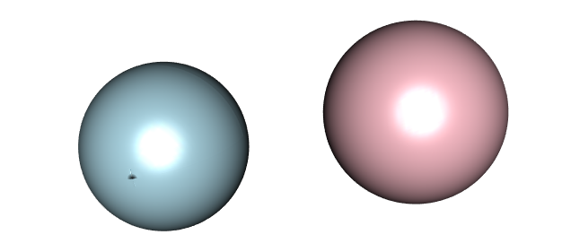
Expanding on cuttlefish44's excellent answer, I found a parameterization that works better - i.e. it has no defect at the poles (the black artifact on the lightblue sphere in the image).

library(rgl)
sphere.f <- function(x0 = 0, y0 = 0, z0 = 0, r = 1, n = 101, ...){
  f <- function(s, t) cbind(r * cos(s) * cos(t) + x0,
                            r * sin(s) * cos(t) + y0, 
                            r * sin(t) + z0)
  persp3d(f, slim = c(0, pi), tlim = c(0, 2*pi), n = n, add = T, ...)
}


sphere1.f <- function(x0 = 0, y0 = 0, z0 = 0, r = 1, n = 101, ...){
  f <- function(s,t){ 
    cbind(   r * cos(t)*cos(s) + x0,
             r *        sin(s) + y0,
             r * sin(t)*cos(s) + z0)
  }
  persp3d(f, slim = c(-pi/2,pi/2), tlim = c(0, 2*pi), n = n, add = T, ...)
}


sphere.f( -1.5,0, col = "lightblue")
sphere1.f( 1.5,0, col = "pink")

The image:

Margarite

This is excellent - good job. At n=101, the ridge defect around the equator is still there, but a good compromise between speed and quality. With n=201, its already hard to see. At n=301, barely discernible and still acceptably fast. – Manos

Thanks for giving me the correct answer vote. Would love to get a bronze badge in rgl, but at this rate it will take about 10 years. – Margarite

Answer 2

A much simpler approach is to use subdivision3d(). Here, depth=4 isn't all that smooth, but you could increase that.

library(rgl)
sphere <- subdivision3d(cube3d(),depth=4)
sphere$vb[4,] <- apply(sphere$vb[1:3,], 2, function(x) sqrt(sum(x^2)))
open3d()
shade3d(sphere, col="red")

Wireman

Adding normals makes it look even better. You can do this by adding sphere$normals <- sphere$vb for a sphere, or more generally shape <- addNormals(shape). – Epithelioma

I like the simplicity of this approach. And it can be improved by using dodecahedron3d() rather than cube3d(). Unfortunately, it does not work for high resolution spheres. If I increase depth above 6 I tend to get memory allocation errors. That said, dodecahedron3d at depth 6 looks pretty passable, if somewhat slow to process – Manos

Further to my last comment, adding @Epithelioma 's suggestion of adding normals to icosahedron3d() subdivided at depth 6, makes some pretty nice looking spheres – Manos

Answer 3

Although rgl::spheres3d() can't do this, an alternative is to write your own function to draw spheres. Here is a function that renders a sphere as a grid of quadrilaterals spaced at equal degrees of latitude and longitude.

drawSphere = function(xc=0, yc=0, zc=0, r=1, lats=50L, longs=50L, ...) {
  #xc,yc,zc give centre of sphere, r is radius, lats/longs for resolution
  vertices = vector(mode = "numeric", length = 12L * lats * longs)
  vi = 1L
  for(i in 1:lats) {
    lat0 = pi * (-0.5 + (i - 1) / lats)
    z0   = sin(lat0)*r
    zr0  = cos(lat0)*r
    lat1 = pi * (-0.5 + i / lats)
    z1   = sin(lat1)*r
    zr1  = cos(lat1)*r
    for(j in 1:longs) {
      lng1 = 2 * pi *  (j - 1) / longs
      lng2 = 2 * pi *  (j) / longs
      x1 = cos(lng1)
      y1 = sin(lng1)
      x2 = cos(lng2)
      y2 = sin(lng2)
      vertices[vi] = x1 * zr0 + xc;    vi = vi + 1L
      vertices[vi] = y1 * zr0 + yc;    vi = vi + 1L 
      vertices[vi] = z0 + zc;          vi = vi + 1L
      vertices[vi] = x1 * zr1 + xc;    vi = vi + 1L
      vertices[vi] = y1 * zr1 + yc;    vi = vi + 1L
      vertices[vi] = z1 + zc;          vi = vi + 1L
      vertices[vi] = x2 * zr1 + xc;    vi = vi + 1L
      vertices[vi] = y2 * zr1 + yc;    vi = vi + 1L
      vertices[vi] = z1 + zc;          vi = vi + 1L
      vertices[vi] = x2 * zr0 + xc;    vi = vi + 1L
      vertices[vi] = y2 * zr0 + yc;    vi = vi + 1L
      vertices[vi] = z0 + zc;          vi = vi + 1L
    }
  }
  indices = 1:(length(vertices)/3)
  shade3d(qmesh3d(vertices, indices, homogeneous=F), ...)
}

It should be possible to improve on this, for example using icospheres (i.e. drawing the sphere as a stretched icosohedron). But this version already draws pretty good spheres if you make lats and longs high enough.

An example of the function in action:

spheres = data.frame(x = c(1,2,3), y = c(1,3,1), z=c(0,0,0), color = c("#992222" , "#222299", "#229922"))
open3d() 
material3d(ambient = "black", specular = "grey60", emission = "black", shininess = 30.0)
rgl.clear(type = "lights")
rgl.light(theta = -30, phi = 60, viewpoint.rel = TRUE, ambient = "#FFFFFF", diffuse = "#FFFFFF", specular = "#FFFFFF", x = NULL, y = NULL, z = NULL)
rgl.light(theta = -0, phi = 0, viewpoint.rel = TRUE,  diffuse = "gray20", specular = "gray25", ambient = "gray80", x = NULL, y = NULL, z = NULL)
sapply(1:NROW(spheres), function(i) 
  drawSphere(spheres$x[i], spheres$y[i], spheres$z[i], r=1, lats = 400, longs = 400, color=spheres$color[i]))

Manos

Yes, drawing your own sphere is the way to go. One possible improvement if you want just one colour is that you can draw just one sphere, and reuse it as a 3d sprite. That saves memory, which probably doesn't matter in R, but will make a noticeable difference in file size if you export the scene using rglwidget(). – Epithelioma

Answer 4

Here is my approach using persp3d.function()

sphere.f <- function(x0 = 0, y0 = 0, z0 = 0, r = 1, n = 101, ...){
  f <- function(s, t) cbind(r * cos(s) * cos(t) + x0,
                            r * sin(s) * cos(t) + y0, 
                            r * sin(t) + z0)
  persp3d(f, slim = c(0, pi), tlim = c(0, 2*pi), n = n, add = T, ...)
}

sphere.f(col = rainbow)

Current

This makes some very nice smooth looking spheres, and is significantly faster to process than my qmesh3d based function. The one thing holding me back from accepting this answer is that the spheres have defects around the poles, where there are gaps in the surface, and also a slight ridge at the equator where the two hemispheres don't quite match up. Do you have any ideas about how to fix these issues? – Manos

@dww; Unfortunately it seems impossible. There some methods to express sphere with two variables. But low or high density area and/or duplicated points arise in any way. – Current

Answer 5

It's not easy; I think if you want to do this you're going to have to

• download the rgl source from CRAN
• unpack it and modify line 24 of src/sphereSet.cpp, which is currently

sphereMesh.setGlobe(16,16);

to call the function with some larger values (this function is defined on line 25 of src/SphereMesh.cpp; the arguments are in_segments and in_sections ...)

• build/install the package from source; this will require not only the standard compilation tools, but also the relevant OpenGL libraries (on a Debian Linux OS you could use sudo apt-get build-dep r-cran-rgl to get them, I think ...)

I haven't tried this. Good luck ... alternately, you could ask the package maintainer to make this a settable parameter via materials3d or in some other way ...

Busboy

I would try downloading the source, editing the line mentioned above and the DESCRIPTION file (to set yourself to be the maintainer), and upload it up via ftp to win-builder.r-project.org – Busboy

Answer 6

Another possibility is to use the vcgSphere function of the Rvcg package.

library(Rvcg)
sphr <- vcgSphere(subdivision = 4) # unit sphere centered at (0,0,0)
library(rgl)
shade3d(sphr, color="red")

# sphere with given radius and center
radius <- 0.5
center <- c(2,1,1)
sphr2 <- translate3d(
  scale3d(sphr, radius, radius, radius), 
  center[1], center[2], center[3])
shade3d(sphr2, color="green")

Historic