averaging mask and laplacian mask in image processing

Question

in a given application I apply an averaging mask to input images to reduce noise, and then a Laplacian mask to enhance small details. Anyone knows if I Would get the same results if I reverse the order of these operations in Matlab?

Bearded

Answer 1

Convolving with a Laplacian kernel is similar to using second derivative information about the intensity changes. Since this derivative is sensitive to noise, we often smooth the image with a Gaussian before applying the Laplacian filter.

---

Here's a MATLAB example similar to what @belisarius posted:

f='http://upload.wikimedia.org/wikipedia/commons/f/f4/Noise_salt_and_pepper.png';
I = imread(f);

kAvg = fspecial('average',[5 5]);
kLap = fspecial('laplacian',0.2);

lapMask = @(I) imsubtract(I,imfilter(I,kLap));

subplot(131), imshow(I)
subplot(132), imshow( imfilter(lapMask(I),kAvg) )
subplot(133), imshow( lapMask(imfilter(I,kAvg)) )

Friulian

NICE Thank you! so what happenned when the procedures were reversed? – Bearded

@biz: 'thron of three' explained it well, refer to his answer – Friulian

Answer 2

Lets say you have two filters F1 and F2, and an image I. If you pass your image through the two filters, you would get a response that was defined as

X = ((I * F1) * F2)

Where here I am using * to represent convolution.

By the associative rule of convolution, this is the same as.

X = (I * (F1 * F2))

using commutativity, we can say that

X = (I * (F2 * F1)) = ((I * F2) * F1)

Of course, this is in the nice continuous domain of math, doing these things on a machine means there will be rounding errors and some data may be lost. You also should think about if your filters are FIR, otherwise the whole concept of thinking about digital filtering as convolution sorta starts to break down as your filter can't really behave the way you wanted it to.

---

EDIT

The discrete convolution is defined as

so adding zeros at the edges of you data doesn't change anything in a mathematical sense.

As some people have pointed out, you will get different answers numerically, but this is expected whenever we deal with computing actual data. These variations should be small and limited to the low energy components of the output of the convolution (i.e: the edges).

It is also important to consider how the convolution operation is working. Convolving two sets of data of length X and length Y will result in an answer that is X+Y-1 in length. There is some behind the scenes magic going on for programs like MATLAB and Mathematica to give you an answer that is of length X or Y.

So in regards to @belisarius' post, it would seem we are really saying the same thing.

Gerson

Applying image filters usually require some padding (particularly set for each filter, depending on the values on the image boundary). And that breaks the commutation property. – Taking

@belisarius I am not sure I am following how padding (zero or otherwise) would break the commutative property for convolution. Can you provide a proof? – Gerson

@belisarius I think we might be saying the same thing here. See my edits. – Gerson

Answer 3

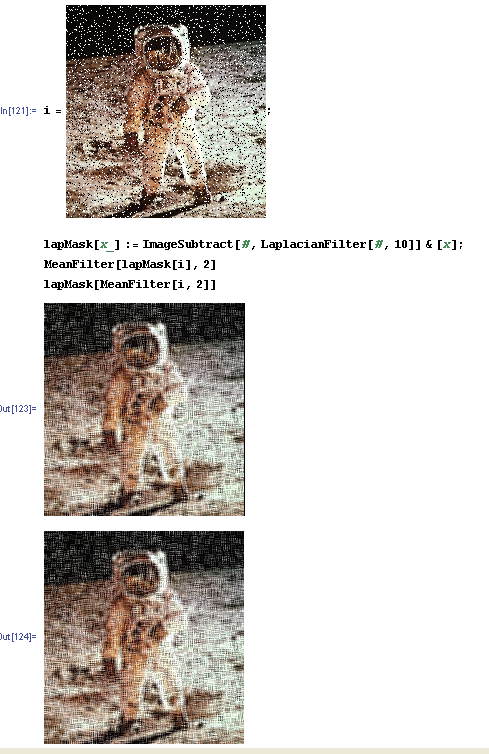
Numerically the results are not the same, but the images look pretty similar.

Example in Mathematica:

Edit

As an answer to @thron comment in his answer about commutation of linear filters and padding, just consider the following operations.

While commutation of a Gaussian and Laplacian filter without padding is true:

list = {1, 3, 5, 7, 5, 3, 1};
gauss[x_] := GaussianFilter[ x, 1]
lapl[x_] := LaplacianFilter[x, 1]
Print[gauss[lapl[list]], lapl[gauss[list]]]
(*
->{5.15139,0.568439,-1.13688,-9.16589,-1.13688,0.568439,5.15139}    
  {5.15139,0.568439,-1.13688,-9.16589,-1.13688,0.568439,5.15139}
*)

Doing the same with padding, result in a difference at the edges:

gauss[x_] := GaussianFilter[ x, 1, Padding -> 1]
lapl[x_] := LaplacianFilter[x, 1, Padding -> 1]
Print[gauss[lapl[list]], lapl[gauss[list]]]

(*
->{4.68233,0.568439,-1.13688,-9.16589,-1.13688,0.568439,4.68233}
  {4.58295,0.568439,-1.13688,-9.16589,-1.13688,0.568439,4.58295}
*)

Taking

wow Thanks a lot if it is not too much asked, can you do an exemple in Matlab? – Bearded

@biz Sorry, I don't have Matlab available. I'm sure other members can post it. HTH! – Taking