Speed up Metropolis-Hastings algorithm in Python

Question

I have some code that samples a posterior distribution using MCMC, specifically Metropolis Hastings. I use scipy to generate random samples:

import numpy as np
from scipy import stats

def get_samples(n):
    """
    Generate and return a randomly sampled posterior.

    For simplicity, Prior is fixed as Beta(a=2,b=5), Likelihood is fixed as Normal(0,2)

    :type n: int
    :param n: number of iterations

    :rtype: numpy.ndarray
    """
    x_t = stats.uniform(0,1).rvs() # initial value
    posterior = np.zeros((n,))
    for t in range(n):
        x_prime = stats.norm(loc=x_t).rvs() # candidate
        p1 = stats.beta(a=2,b=5).pdf(x_prime)*stats.norm(loc=0,scale=2).pdf(x_prime) # prior * likelihood 
        p2 = stats.beta(a=2,b=5).pdf(x_t)*stats.norm(loc=0,scale=2).pdf(x_t) # prior * likelihood 
        alpha = p1/p2 # ratio
        u = stats.uniform(0,1).rvs() # random uniform
        if u <= alpha:
            x_t = x_prime # accept
            posterior[t] = x_t
        elif u > alpha:
            x_t = x_t # reject
    posterior = posterior[np.where(posterior > 0)] # get rid of initial zeros that don't contribute to distribution
    return posterior

Generally, I try to avoid using explicit for loops in python - I would try to generate everything using pure numpy. For the case of this algorithm however, a for loop with if statements is unavoidable. Therefore, the code is quite slow. When I profile my code, it is spending most time within the for loop (obviously), and more specifically, the slowest parts are in generating the random numbers; stats.beta().pdf() and stats.norm().pdf().

Sometimes I use numba to speed up my code for matrix operations. While numba is compatible with some numpy operations, generating random numbers is not one of them. Numba has a cuda rng, but this is limited to normal and uniform distributions.

My question is, is there a way to significantly speed up the code above using some sort of random sampling of various distributions compatible with numba?

We don't have to limit ourselves to numba, but it is the only easy to use optimizer that I know of. More generally, I am looking for ways to speed up random sampling for various distributions (beta, gamma, poisson) within a for loop in python.

Distance

Numba supports quite a lot random distributions. numba.pydata.org/numba-doc/dev/reference/… I guess the main thing you have to implement yourself is the pdf method (github.com/scipy/scipy/blob/v1.2.1/scipy/stats/…) – Warily

stats.beta().pdf() and stats.norm().pdf() are not generating random numbers. They're evaluating the density of the probability distributions. – Aam

BTW if you look in the scipy-source code you will find calls to scipy.special functions (xlog1py, betaln). This is an easy way to make them available within Numba github.com/numba/numba/issues/3086 – Warily

Answer 1

There are lots of optimisations you can make to this code before you start thinking about numba et. al. (I managed to get a 25x speed up on this code only by being smart with the algorithm's implementation)

Firstly, there's an error in your implementation of the Metropolis--Hastings algorithm. You need to keep every iteration of the scheme, regardless of whether your chain moves or not. That is, you need to remove posterior = posterior[np.where(posterior > 0)] from your code and at the end of each loop have posterior[t] = x_t.

Secondly, this example seems odd. Typically, with these kinds of inference problems we're looking to infer the parameters of a distribution given some observations. Here, though, the parameters of the distribution are known and instead you're sampling observations? Anyway, whatever, regardless of this I'm happy to roll with your example and show you how to speed it up.

Speed-up

To get started, remove anything which is not dependent on the value of t from the main for loop. Start by removing the generation of the random walk innovation from the for loop:

    x_t = stats.uniform(0,1).rvs()
    innov = stats.norm(loc=0).rvs(size=n)
    for t in range(n):
        x_prime = x_t + innov[t]

Of course it is also possible to move the random generation of u from the for loop:

    x_t = stats.uniform(0,1).rvs()
    innov = stats.norm(loc=0).rvs(size=n)

    u = np.random.uniform(size=n)
    for t in range(n):
        x_prime = x_t + innov[t]
        ...
        if u[t] <= alpha:

Another issue is that you're computing the current posterior p2 in every loop, which isn't necessary. In each loop you need to calculate the proposed posterior p1, and when the proposal is accepted you can update p2 to equal p1:

    x_t = stats.uniform(0,1).rvs()
    innov = stats.norm(loc=0).rvs(size=n)

    u = np.random.uniform(size=n)

    p2 = stats.beta(a=2,b=5).pdf(x_t)*stats.norm(loc=0,scale=2).pdf(x_t)
    for t in range(n):
        x_prime = x_t + innov[t]

        p1 = stats.beta(a=2,b=5).pdf(x_prime)*stats.norm(loc=0,scale=2).pdf(x_prime)
        ...
        if u[t] <= alpha:
            x_t = x_prime # accept
            p2 = p1

        posterior[t] = x_t

A very minor improvement could be in importing the scipy stats functions directly into the name space:

from scipy.stats import norm, beta

Another very minor improvement is in noticing that the elif statement in your code doesn't do anything and so can be removed.

Putting this altogether and using more sensible variable names I came up with:

from scipy.stats import norm, beta
import numpy as np

def my_get_samples(n, sigma=1):

    x_cur = np.random.uniform()
    innov = norm.rvs(size=n, scale=sigma)
    u = np.random.uniform(size=n)

    post_cur = beta.pdf(x_cur, a=2, b=5) * norm.pdf(x_cur, loc=0, scale=2)

    posterior = np.zeros(n)
    for t in range(n):
        x_prop = x_cur + innov[t]

        post_prop = beta.pdf(x_prop, a=2, b=5) * norm.pdf(x_prop, loc=0, scale=2)
        alpha = post_prop / post_cur
        if u[t] <= alpha:
            x_cur = x_prop
            post_cur = post_prop

        posterior[t] = x_cur

    return posterior

Now, for a speed comparison:

%timeit get_samples(1000)
3.19 s ± 5.28 ms per loop (mean ± std. dev. of 7 runs, 1 loop each)
%timeit my_get_samples(1000)
127 ms ± 484 µs per loop (mean ± std. dev. of 7 runs, 10 loops each)

That's a speed up of 25x

ESS

It's worth noting that brute speed isn't everything when it comes to MCMC algorithms. Really, what you're interested in is the number of independent(ish) draws you can make from the posterior per second. Typically, this is assessed with the ESS (effective sample size). You can improve the efficiency of your algorithm (and hence increase your effective samples drawn per second) by tuning your random walk.

To do so it is typical to make an initial trial run, i.e. samples = my_get_samples(1000). From this output calculate sigma = 2.38**2 * np.var(samples). This value should then be used to tune the random walk in your scheme as innov = norm.rvs(size=n, scale=sigma). The seemingly arbitrary occurrence of 2.38^2 has it's origin in:

Weak convergence and optimal scaling of random walk Metropolis algorithms (1997). A. Gelman, W. R. Gilks, and G. O. Roberts.

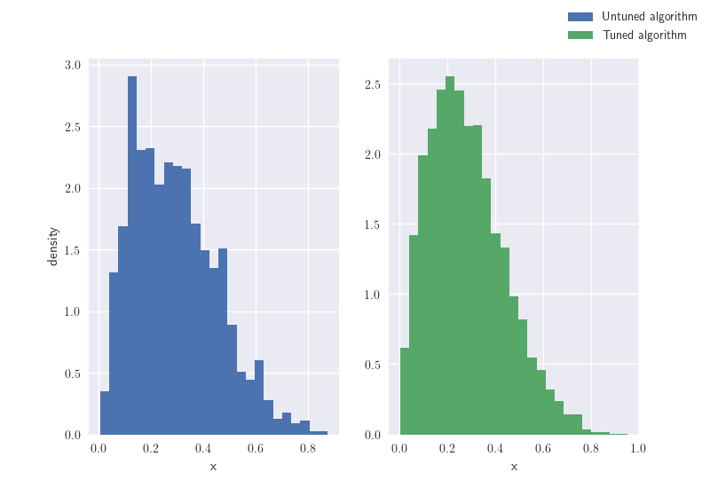
To illustrate the improvements tuning can make let's make two runs of my algorithm, one tuned and the other untuned, both using 10000 iterations:

x = my_get_samples(10000)
y = my_get_samples(10000, sigma=0.12)

fig, ax = plt.subplots(1, 2)
ax[0].hist(x, density=True, bins=25, label='Untuned algorithm', color='C0')
ax[1].hist(y, density=True, bins=25, label='Tuned algorithm', color='C1')
ax[0].set_ylabel('density')
ax[0].set_xlabel('x'), ax[1].set_xlabel('x')
fig.legend()

You can immediately see the improvements tuning has made to our algorithm's efficiency. Remember, both runs were made for the same number of iterations.

Final thoughts

If your algorithm is taking a very long time to converge, or if your samples have large amounts of autocorrelation, I'd consider looking into Cython to squeeze out further speed optimisations.

I'd also recommend checking out the PyStan project. It takes a bit of getting used to, but its NUTS HMC algorithm will likely outperform any Metropolis--Hastings algorithm you can write by hand.

Aam

If you set np.random.seed() to a specific state, the results should be the same, but they are not. Thus your function does not yield the same result as the function in the question. – Sensitometer

Of course the samples returned are not exactly the same. The order in which the random numbers are generated are completely different. – Aam

The way to check that the results are the same is to verify that both algorithms have converged to the same posterior distribution. I.e. something like x = get_samples(10000) y = my_get_samples(10000) plt.hist(x); plt.hist(y) – Aam

I'm not an expert in statistics, nor in how np.random.seed behaves internally, but imho using a fixed seed should yield exactly the same result. – Sensitometer

You're right, setting the seed ensures the same numbers are returned but only if the numbers are generated in the same order. Consider the following snippet: np.random.seed(1) x1 = np.zeros(10); y1 = np.zeros(10) for i in range(10): x1[i] = np.random.uniform(); y1[i] = np.random.uniform() np.random.seed(1) x2 = np.random.uniform(size=10); y2 = np.random.uniform(size=10) The variables x1 and x2 are generated with the same seed, but because the order in which they're generated has changed if you inspect the objects you'll see they're not the same. – Aam

Ok, I see that you are right. :) But still I think that outsourcing p2 (or post_cur in your case) is not correct, since x_cur/x_t changes in some iterations of the loop. Or is this covered with innov? – Sensitometer

If x_cur changes (i.e. the proposal is accepted), then I update post_cur = post_prop in the if statement. You can check this is true by fixing the random seed and trying my code with post_cur in and out of the loop. The output will be the same. – Aam

Oh right, didn't see that you also update post_cur. Thanks for clarification. I guess you deserve an upvote and having your answer accepted. :) – Sensitometer

good implementation, thanks for that! it does speed it up a lot. now I need to find a way to use a pdf method compatible with numba as you commented on my question – Distance

You're welcome. Before you look into numba you first should tune the random walk of your scheme. I'm adding some more info to my answer now. – Aam

@jwalton3141, not that it will contribute to the performance, but it may help to include one more line of code before we return posterior. I was thinking to thin the samples to reduce autocorrelation and also only take samples from say 1000 onwards (burn in period) to remove the initial random samples: posterior = posterior[1000::4] # use 1000 onwards (burn in) and take every 4th sample (thinning) – Distance

@Jack would you be able to comment on PyRsquared comment? I was reading Monte Carlo Statistical Methods by Casella and Pattern Recognition and Machine Learning by Bishop and both suggest using a burn-in period and to get every Mth sample. Would posterior[burn_in::M] do the job? – Schnur

@Schnur posterior[burn_in::M] would do what you desire. Personally, unless memory is an issue, I'd return posterior from get_samples, inspect the output with trace plots, autocorrelation plots etc. and only then decide how much burn-in and thinning to add. See how this differs from PyRsquared's suggestions to return posterior[burn_in::M] from get_samples --- in this case we'd be deciding a burn-in period and thinning without seeing the full output. – Aam

@Jack that is quite sensible. Thanks a lot! – Schnur

Answer 2

Unluckily I really don't see any possibility to speed up the random distributions, except for rewriting them yourself in numba compatible python code.

But one easy possibility to speed up the bottleneck of your code, is to replace the two calls to the stats functions to one call with:

p1, p2 = (
    stats.beta(a=2, b=5).pdf([x_prime, x_t])
    * stats.norm(loc=0, scale=2).pdf([x_prime, x_t])
)

Another slight tweak may be outsourcing the generation of u outside of the for loop with:

x_t = stats.uniform(0, 1).rvs() # initial value
posterior = np.zeros((n,))
u = stats.uniform(0, 1).rvs(size=n) # random uniform
for t in range(n):  # and so on

And then indexing u within the loop (of course the line u = stats.uniform(0,1).rvs() # random uniform in the loop has to be deleted):

if u[t] <= alpha:
    x_t = x_prime # accept
    posterior[t] = x_t
elif u[t] > alpha:
    x_t = x_t # reject

Minor changes may also be simplifying the if condition by omitting the elif statement or if required for other purposes by replacing it with else. But this is really just a tiny improvement:

if u[t] <= alpha:
    x_t = x_prime # accept
    posterior[t] = x_t

Edit

Another improvement based on jwalton's answer:

def new_get_samples(n):
    """
    Generate and return a randomly sampled posterior.

    For simplicity, Prior is fixed as Beta(a=2,b=5), Likelihood is fixed as Normal(0,2)

    :type n: int
    :param n: number of iterations

    :rtype: numpy.ndarray
    """
    
    x_cur = np.random.uniform()
    innov = norm.rvs(size=n)
    x_prop = x_cur + innov
    u = np.random.uniform(size=n)

    post_cur = beta.pdf(x_cur, a=2,b=5) * norm.pdf(x_cur, loc=0,scale=2)
    post_prop = beta.pdf(x_prop, a=2,b=5) * norm.pdf(x_prop, loc=0,scale=2)

    posterior = np.zeros((n,))
    for t in range(n):        
        alpha = post_prop[t] / post_cur
        if u[t] <= alpha:
            x_cur = x_prop[t]
            post_cur = post_prop[t]
        posterior[t] = x_cur
    return posterior

With the improved timings of:

%timeit my_get_samples(1000)
# 187 ms ± 13 ms per loop (mean ± std. dev. of 7 runs, 10 loops each)
%timeit my_get_samples2(1000)
# 1.55 ms ± 57.3 µs per loop (mean ± std. dev. of 7 runs, 1000 loops each)

This is a speed-up of a factor of 121 over jwalton's answer. It is accomplished by outsourcing post_prop calculation.

Checking the histogram, this seems to be ok. But better ask jwalton if it really is ok, he seems to have much more understanding of the topic. :)

Sensitometer