multi-sensors fusion using Kalman filter

Question

I need to use the Kalman filter to fuse multi-sensors positions for gaussian measurement (for example 4 positions as the input of the filter and 1 position as output). It is possible to help me with some examples or tutorials because all the examples I found are related to the estimation of the positions?

Grannie

dsp.stackexchange.com/questions/85434/… – Arst

Answer 1

OPTION 1

Weighted Avarage

In this case you don't need to implement a real Kalman Filter. You just can use the signal variances to calculate the weights and then calculate the weighted avarage of the inputs. The weights can be found as an inverse of the variances.

So if you have two signals S1 and S2 with variances V1 and V2, then the fused result would be

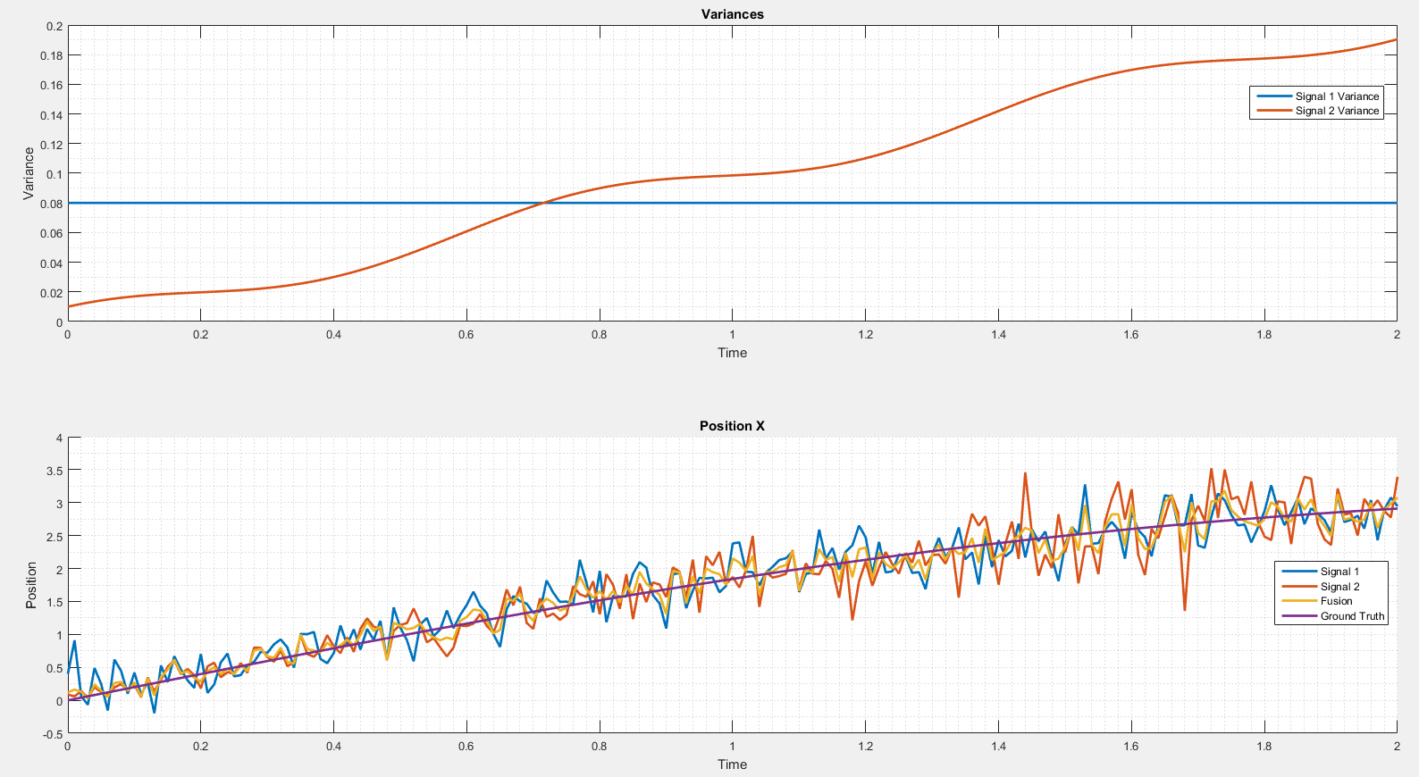
A fusion example can be seen on the next plot.

I simulated two signals. The variance of the second signal changes over the time. As long as it's smaller than the variance of the first signal the fused result is close to the second signal. It is not the case when the variance of the second signal is too high.

OPTION 2

Kalman Filter with Multiple Update Steps

The classical Kalman Filter uses prediction and update steps in a loop:

prediction 
update
prediction 
update
...

In your case you have 4 independent measurements, so you can use those readings after each other in separate update steps:

prediction 
update 1
update 2
update 3
update 4
prediction 
update 1
...

A very nice point is that the order of those updates does not matter! You can use updates 1,2,3,4 or 3,2,4,1. In both cases you should get the same fused output.

Compared to the first option you have following pros:

• You have a variance propogation
• You have the system noise matrix Q, so you can control the smoothness of the fused output

Here is my matlab code:

function [] = main()
    % time step
    dt = 0.01;

    t=(0:dt:2)';
    n = numel(t);

    %ground truth
    signal = sin(t)+t; 

    % state matrix
    X = zeros(2,1);

    % covariance matrix
    P = zeros(2,2);

    % kalman filter output through the whole time
    X_arr = zeros(n, 2);

    % system noise
    Q = [0.04 0;
         0 1];

    % transition matrix
    F = [1 dt;
         0 1]; 

    % observation matrix 
    H = [1 0];

    % variance of signal 1 
    s1_var = 0.08*ones(size(t)); 
    s1 = generate_signal(signal, s1_var);

    % variance of signal 2 
    s2_var = 0.01*(cos(8*t)+10*t);
    s2 = generate_signal(signal, s2_var);

    % variance of signal 3 
    s3_var = 0.02*(sin(2*t)+2);
    s3 = generate_signal(signal, s3_var);

    % variance of signal 4 
    s4_var = 0.06*ones(size(t)); 
    s4 = generate_signal(signal, s4_var);

    % fusion
    for i = 1:n
        if (i == 1)
            [X, P] = init_kalman(X, s1(i, 1)); % initialize the state using the 1st sensor
        else
            [X, P] = prediction(X, P, Q, F);

            [X, P] = update(X, P, s1(i, 1), s1(i, 2), H);
            [X, P] = update(X, P, s2(i, 1), s2(i, 2), H);
            [X, P] = update(X, P, s3(i, 1), s3(i, 2), H);
            [X, P] = update(X, P, s4(i, 1), s4(i, 2), H);
        end

        X_arr(i, :) = X;
    end

    plot(t, signal, 'LineWidth', 4);
    hold on;
    plot(t, s1(:, 1), '--', 'LineWidth', 1);
    plot(t, s2(:, 1), '--', 'LineWidth', 1);
    plot(t, s3(:, 1), '--', 'LineWidth', 1);
    plot(t, s4(:, 1), '--', 'LineWidth', 1);
    plot(t, X_arr(:, 1), 'LineWidth', 4);
    hold off;
    grid on;
    legend('Ground Truth', 'Sensor Input 1', 'Sensor Input 2', 'Sensor Input 3', 'Sensor Input 4', 'Fused Output');
end

function [s] = generate_signal(signal, var)
    noise = randn(size(signal)).*sqrt(var);

    s(:, 1) = signal + noise;
    s(:, 2) = var; 
end

function [X, P] = init_kalman(X, y)
    X(1,1) = y;
    X(2,1) = 0;

    P = [100 0;
         0   300];
end

function [X, P] = prediction(X, P, Q, F)
    X = F*X;
    P = F*P*F' + Q;
end

function [X, P] = update(X, P, y, R, H)
    Inn = y - H*X;
    S = H*P*H' + R;
    K = P*H'/S;

    X = X + K*Inn;
    P = P - K*H*P;
end

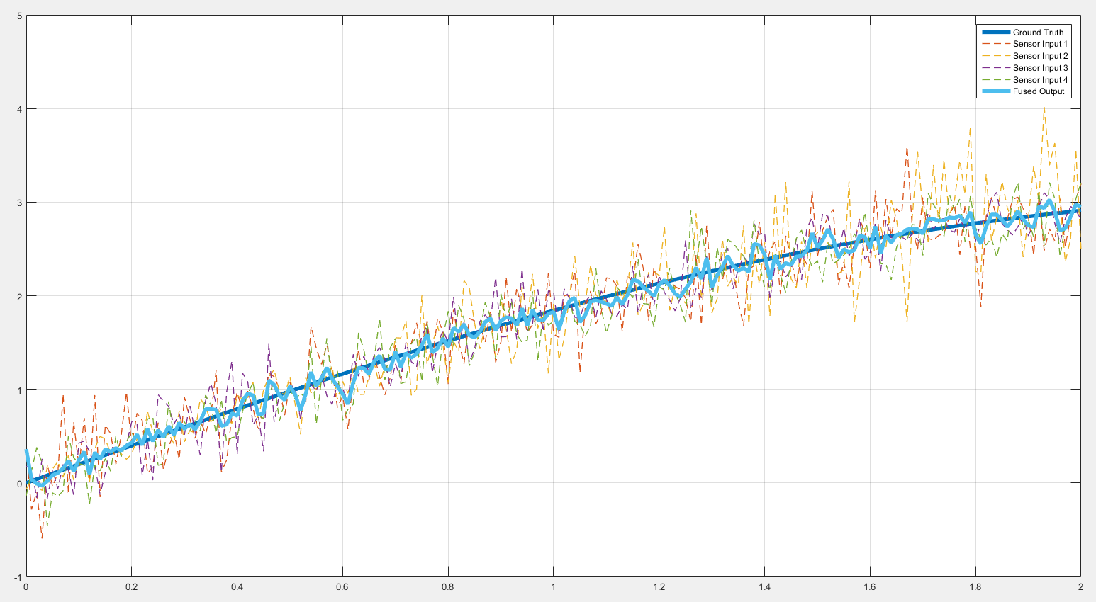
And here is the result:

Trubow

Thank you for replying but in this case, we are not in the MLE (mean likelihood estimation) case? so how to update the variances? – Grannie

Have a look at Option 2. I think this is a better way with some advantages. – Trubow

Thank you it is so helpful. – Grannie

Very helpful indeed, thanks. Can the update step be done for multiple sensors in one matrix calculation? – Inessa

Unfortunately no, you need to iterate through the measurements separately. From the filter "point view" there is only one sensor and only one measurement at a time. But it is a nice thing because you can work with a number of sensors in a generic way. if at some point only two out of four measurements are available you don't need to customize your model, you just iterate through those two sensors and ignore the others. – Trubow

@Trubow Why can't you update multiple sensors in one matrix calculation? Can't you just make H = [1 0; 1 0; 1 0; 1 0] and R = diag([var1 var2 var3 var4]) and run just one update step? – Mooring

I like the idea of being able to run multiple update steps though. Seems like it could be more computationally efficient for lots of redundant sensors. – Mooring

"In your case you have 4 independent measurements, so you can use those readings after each other in separate update steps“ . I am curious? Why is that the case? – Loewi

I'm wondering if the update order does not matter, is there a way to "reduce" the 4 measurements into 1 and update that? My tests seem to suggest that reduce by averaging nor summation both give different final results. – Vital