How to set boundary condition in a complex soap film GAM smoother?

I am modelling the distribution of bottlenose dolphins in the lagoon of a South Pacific Island. I would like to use a soap-film smoother to model the probability of dolphin presence over a 2D surface (longitude x latitude) accounting for land boundaries (as obviously dolphins cannot go on land).

I woukd like to know how to fix the boundary of my study area (land and offshore waters) to a condition equal to zero, as I am expecting to have a null probability of finding a dolphin on land, as well as in the most offshore waters of my study area (this species of dolphin is only found in lagoon shallow waters). So far, I have tested several approaches that I will describe below, but the maps predicted by my models do not follow my expectations as to how the boundary condition should be handled.

Here is what the dataset looks like when mapped. Dolphin locations are shown in blue, while absence locations are shown in pink. The land is shown in black and the reefs delineating the lagoon in grey.

Step 1: create the boundary and knots objects

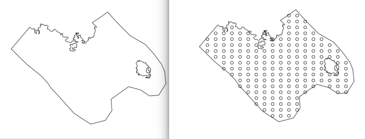
I created a boundary polygon called soap_bnd, converted it to a list of lists called bound and filled it with knots soap_knots. The boundary includes two inner "holes" that are formed by two islands found in the study area. The following code was inspired by: Gavin Simpson's excellent blogpost https://www.fromthebottomoftheheap.net/2016/03/27/soap-film-smoothers/ and https://journals.plos.org/plosone/article/file?type=supplementary&id=info:doi/10.1371/journal.pone.0205921.s001 I use the function autocrunch created by David L Miller (see https://github.com/dill/soap_checker).

Positions are in a projected UTM coordinate system (hence the coordinate columns are called utmx and utmy)

## boundary of the soap film (one polygon with two inner loops)
# soap_bnd is initially a SpatialPolygonDataFrame
crds <- tidy(soap_bnd)
crds <- crds %>% dplyr::select(long, lat, piece)
names(crds) <- c("x", "y", "piece")
bound <- split(crds, crds$piece)
bound <-lapply(bound,`[`, c(1, 2))
nr <- seq(1, 3)
bound <-lapply(nr, function(n) as.list.data.frame(bound[[n]]))

## bound is a list of 3 lists (because 1 large polygon and 2 loops), each including 3 elements (utmx, utmy and f)
## an element f is set to a vector of zeros to set the boundary condition
bound <- lapply(nr, function(n) bound[[n]] <- c(bound[[n]], list(f = rep(0, length(bound[[n]]$x)))))

## created a grid of knots within the boundary
soap_knots <- make.soapgrid(bound[[1]][c("x", "y")], 20)

# removing the knots that overlap with the inner loops (the islands)
x <- soap_knots$x
y <- soap_knots$y
soap_knots <- soap_knots[!inSide(x = x, y = y, bnd = bound[[2]]) & 
                           !inSide(x = x, y = y, bnd = bound[[3]]),]

# just changing names so everything matches
bound <- llply(bound, function(b){names(b)[1:2] <- c("utmx", "utmy"); return(b)})
names(soap_knots) <- c("utmx", "utmy")

# remove points too close to the boundary
crunch_ind <- autocruncher(bound, soap_knots, k = 20, xname = "utmx", yname = "utmy")
soap_knots <- soap_knots[-crunch_ind, ]

## plotting the final product
plot(soap_bnd)
points(soap_knots)

Step 2: run the GAM

The GAM model is binomial as I am modeling the distribution of dolphin locations (1) with other locations from which dolphins were absent (0).

m1.1 <- mgcv::gam(response ~ 
                    s(utmx, utmy, bs = "so", xt = list(bnd = bound)),
                    knots = soap_knots,
                    family = binomial, method = "REML", 
                    data = target_df)

# predict the probability of presence using a raster stack called envLS_stack (which includes other environmental variables which are not used here)
pred_ras <- raster::predict(envLS_stack[[c("utmx", "utmy")]], m1.1, type = "response")

# plot the predictions - included between zero (low probability of presence) and one (high probability of presence)
plot(pred_ras, col = rev(brewer.pal(11, "Spectral")), axes = F)

Tests and issues

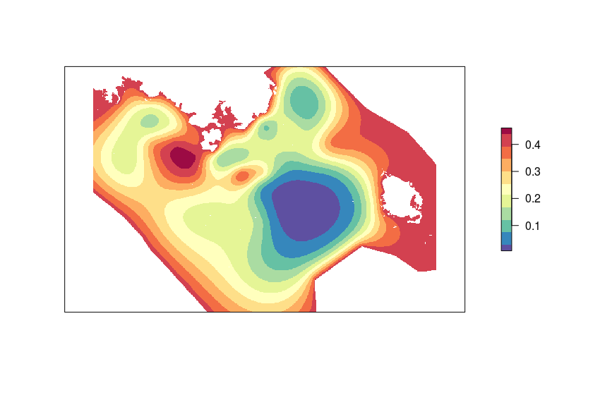
Here is the probability of dolphin presence (lands and offshore waters in white).

I don't understand why the probability on the boundaries turns out being the highest although I set the f boundary to zero.

I tried another approach where I removed the f elements in my bound lists. I rerun the GAM with the following code:

bound_nof <- llply(bound, function(d){list(utmx = d$utmx, utmy = d$utmy)})

# I tried this model with k = 20 or k = 60
m1.2 <- mgcv::gam(response ~ 
                    s(utmx, utmy, k = 20, bs = "so", xt = list(bnd = bound_nof)), 
                    knots = soap_knots,
                    family = binomial, method = "REML", 
                    data = target_df)

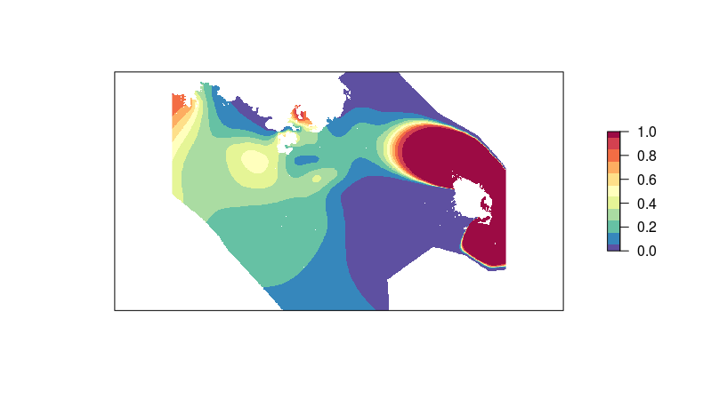
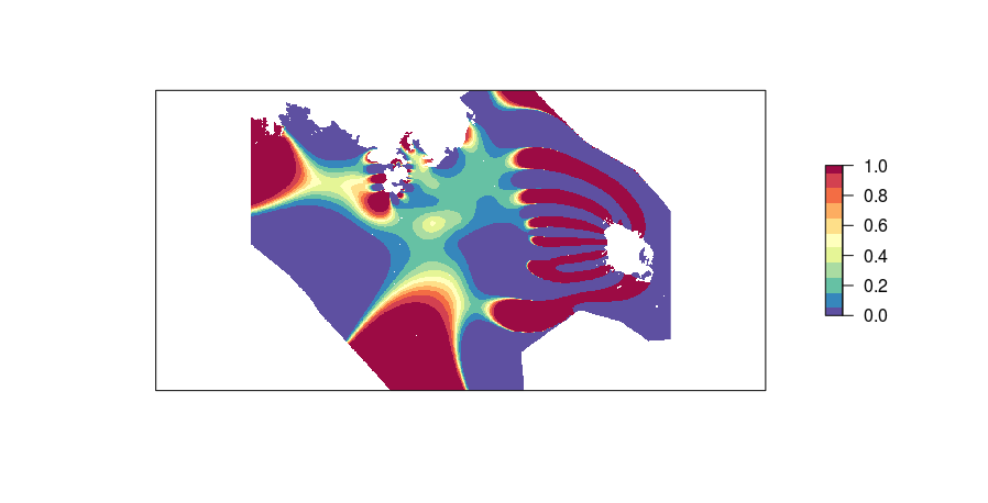
And here is what I get, respectively when using k=20 and k=60:

I cannot figure out what is going on here? In the first map (k=20) it looks like the model strongly picked up on a single dolphin observation made to the extreme west part of the study area and produced a big patch of high probability of presence there... statistically speaking I do not think this pattern is relevant. The second map (k=60) is even more puzzling...

I imagine this pattern may be due to a lack of data to the west and south of my study area. Is it necessary to reduce the size of the finite area where the soap-film is produced? The drawback is that this would prevent any further extrapolation of the model to the larger area I am interested in.

Recommended topics

Hot tags