Gradient descent impementation python - contour lines

Question

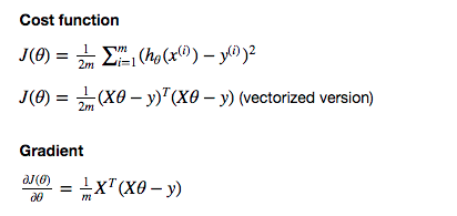
As a self study exercise I am trying to implement gradient descent on a linear regression problem from scratch and plot the resulting iterations on a contour plot.

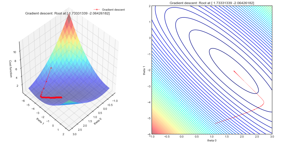
My gradient descent implementation gives the correct result (tested with Sklearn) however the gradient descent plot doesn't seem to be perpendicular to the contour lines. Is this expected or did I get something wrong in my code / understanding?

Algorithm

Cost function and gradient descent

import numpy as np
import pandas as pd
from matplotlib import pyplot as plt
from mpl_toolkits.mplot3d import Axes3D

def costfunction(X,y,theta):
    m = np.size(y)

    #Cost function in vectorized form
    h = X @ theta
    J = float((1./(2*m)) * (h - y).T @ (h - y));    
    return J;


def gradient_descent(X,y,theta,alpha = 0.0005,num_iters=1000):
    #Initialisation of useful values 
    m = np.size(y)
    J_history = np.zeros(num_iters)
    theta_0_hist, theta_1_hist = [], [] #For plotting afterwards

    for i in range(num_iters):
        #Grad function in vectorized form
        h = X @ theta
        theta = theta - alpha * (1/m)* (X.T @ (h-y))

        #Cost and intermediate values for each iteration
        J_history[i] = costfunction(X,y,theta)
        theta_0_hist.append(theta[0,0])
        theta_1_hist.append(theta[1,0])

    return theta,J_history, theta_0_hist, theta_1_hist

Plot

#Creating the dataset (as previously)
x = np.linspace(0,1,40)
noise = 1*np.random.uniform(  size = 40)
y = np.sin(x * 1.5 * np.pi ) 
y_noise = (y + noise).reshape(-1,1)
X = np.vstack((np.ones(len(x)),x)).T


#Setup of meshgrid of theta values
T0, T1 = np.meshgrid(np.linspace(-1,3,100),np.linspace(-6,2,100))

#Computing the cost function for each theta combination
zs = np.array(  [costfunction(X, y_noise.reshape(-1,1),np.array([t0,t1]).reshape(-1,1)) 
                     for t0, t1 in zip(np.ravel(T0), np.ravel(T1)) ] )
#Reshaping the cost values    
Z = zs.reshape(T0.shape)


#Computing the gradient descent
theta_result,J_history, theta_0, theta_1 = gradient_descent(X,y_noise,np.array([0,-6]).reshape(-1,1),alpha = 0.3,num_iters=1000)

#Angles needed for quiver plot
anglesx = np.array(theta_0)[1:] - np.array(theta_0)[:-1]
anglesy = np.array(theta_1)[1:] - np.array(theta_1)[:-1]

%matplotlib inline
fig = plt.figure(figsize = (16,8))

#Surface plot
ax = fig.add_subplot(1, 2, 1, projection='3d')
ax.plot_surface(T0, T1, Z, rstride = 5, cstride = 5, cmap = 'jet', alpha=0.5)
ax.plot(theta_0,theta_1,J_history, marker = '*', color = 'r', alpha = .4, label = 'Gradient descent')

ax.set_xlabel('theta 0')
ax.set_ylabel('theta 1')
ax.set_zlabel('Cost function')
ax.set_title('Gradient descent: Root at {}'.format(theta_result.ravel()))
ax.view_init(45, 45)


#Contour plot
ax = fig.add_subplot(1, 2, 2)
ax.contour(T0, T1, Z, 70, cmap = 'jet')
ax.quiver(theta_0[:-1], theta_1[:-1], anglesx, anglesy, scale_units = 'xy', angles = 'xy', scale = 1, color = 'r', alpha = .9)

plt.show()

Surface and contour plots

Comments

My understanding is that the gradient descent follow contour lines perpendicularly. Is this not the case ? Thanks

Delegation

Each step in gradient descent will reduce total fitting error, true, but is not guaranteed to go directly toward a minimum. Consider the case where you physically spiral down a mountain - each step takes you down, but not straight down. If error space is "bumpy" then gradient descent can get stuck in a local error space minimum as well, that is, the steps in gradient descent are towards a lowER error but not necessarily towards the lowEST error. – Lott

Fair enough, but this function is smooth and quadratic, there are no bumps and no local minima... – Delegation

You are correct, and again each step reduces error but the direction is not always directly straight towards the minimum, just towards a lower error. So there is "descent", but not always in a straight line. – Lott

Agreed, my question is more about why the descent is not perpendicular to the contour. It is at an angle w.r.t the contour lines – Delegation

The gradients w.r.t total error are determined individually for each parameter, yet in each step the parameters are all changed simultaneously and not individually. This combined change might not be perpendicular to the contour lines, as you have seen here. – Lott

Answer 1

The problem with the contour graph is that the scales of theta0 and theta1 are different. Just add "plt.axis('equal')" to the contour plot instructions and you will see that the gradient descent is in fact perpendicular to the contour lines.

Contour graph with same scales in both axis

Aphrodite

Answer 2

In general, Gradient Descent do not follow contour lines.

The following of the contour lines hold true only if the components of the gradient vector are exactly the same (in absolute value), which means that the steepness of function at the evaluation point is the same in each dimension.

So, in your case, only if the curves of the contour plot where concentric circles, not ovals.

Araucanian