compare two time series (simulation results)

Question

I want to do unit testing of simulation models and for that, I run a simulation once and store the results (a time series) as reference in a csv file (see an example here). Now when I change my model, I run the simulation again, store the new reults as a csv file as well and then I compare the results.

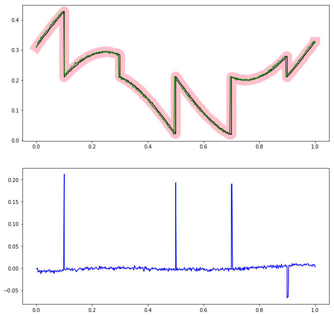
The results are usually not 100% identical, an example plot is shown below:
The reference results are plotted in black and the new results are plotted in green.
The difference of the two is plotted in the second plot, in blue.
As can be seen, at a step the difference can become arbitrarily high, while everywhere else the difference is almost zero.

Therefore, I would prefer to use a different algorithms for comparison than just subtracting the two, but I can only describe my idea graphically: When plotting the reference line twice, first in a light color with a high line width and then again in a dark color and a small line width, then it will look like it has a pink tube around the centerline.

Note that during a step that tube will not only be in the direction of the ordinate axis, but also in the direction of the abscissa. When doing my comparison, I want to know whether the green line stays within the pink tube.

Now comes my question: I do not want to compare the two time series using a graph, but using a python script. There must be something like this already, but I cannot find it because I am missing the right vocabulary, I believe. Any ideas? Is something like that in numpy, scipy, or similar? Or would I have to write the comparison myself?

Additional question: When the script says the two series are not sufficiently similar, I would like to plot it as described above (using matplotlib), but the line width has to be defined somehow in other units than what I usually use to define line width.

Dougie

When you say time series you mean something like a list of [x, y] that can be plot in a 2-D graph? – Maybellmaybelle

Exactly. The reference results and the "new" results are stored as csv files that are read by python, with time being the first column. – Dougie

you could start by looking at their cross-correlation – Beautify

Adding a plot to the question will certainly make it much easier to understand what you are referring to, but it looks like you want some kind of L^2 (or l^2) distance between the two distribution, i.e. something that will be close to zero if the two distribution differ only in at most N number of points (with N finite in the case of continuous distributions). Am I correct? – Quackery

@Quackery Now I have added a plot. – Dougie

What solution was working for you in the end? – Celinecelinka

Dan, unfortunately I did not find a perfect solution, so I continued to use the following two tools: github.com/modelica-tools/csv-compare and github.com/lbl-srg/funnel – Dougie

Answer 1

I would assume here that your problem can be simplified by assuming that your function has to be close to another function (e.g. the center of the tube) with the very same support points and then a certain number of discontinuities are allowed. Then, I would implement a different discretization of function compared to the typical one that is used for L^2 norm (See for example some reference here).

Basically, in the continuous case, the L^2 norm relaxes the constrain of the two function being close everywhere, and allow it to be different on a finite number of points, called singularities This works because there are an infinite number of points where to calculate the integral, and a finite number of points will not make a difference there.

However, since there are no continuous functions here, but only their discretization, the naive approach will not work, because any singularity will contribute potentially significantly to the final integral value.

Therefore, what you could do is to perform a point by point check whether the two functions are close (within some tolerance) and allow at most num_exceptions points to be off.

import numpy as np

def is_close_except(arr1, arr2, num_exceptions=0.01, **kwargs):
    # if float, calculate as percentage of number of points
    if isinstance(num_exceptions, float):
        num_exceptions = int(len(arr1) * num_exceptions)
    num = len(arr1) - np.sum(np.isclose(arr1, arr2, **kwargs))
    return num <= num_exceptions

By contrast the standard L^2 norm discretization would lead to something like this integrated (and normalized) metric:

import numpy as np

def is_close_l2(arr1, arr2, **kwargs):
    norm1 = np.sum(arr1 ** 2)
    norm2 = np.sum(arr2 ** 2)
    norm = np.sum((arr1 - arr2) ** 2)
    return np.isclose(2 * norm / (norm1 + norm2), 0.0, **kwargs)

This however will fail for arbitrarily large peaks, unless you set such a large tolerance than basically anything results as "being close".

Note that the kwargs is used if you want to specify a additional tolerance constraints to np.isclose() or other of its options.

As a test, you could run:

import numpy as np
import numpy.random

np.random.seed(0)

num = 1000
snr = 100
n_peaks = 5
x = np.linspace(-10, 10, num)
# generate ground truth
y = np.sin(x)
# distributed noise
y2 = y + np.random.random(num) / snr
# distributed noise + peaks
y3 = y + np.random.random(num) / snr
peak_positions = [np.random.randint(num) for _ in range(n_peaks)]
for i in peak_positions:
    y3[i] += np.random.random() * snr

# for distributed noise, both work with a 1/snr tolerance
is_close_l2(y, y2, atol=1/snr)
# output: True
is_close_except(y, y2, atol=1/snr)
# output: True

# for peak noise, since n_peaks < num_exceptions, this works
is_close_except(y, y3, atol=1/snr)
# output: True
# and if you allow 0 exceptions, than it fails, as expected
is_close_except(y, y3, num_exceptions=0, atol=1/snr)
# output: False

# for peak noise, this fails because the contribution from the peaks
# in the integral is much larger than the contribution from the rest
is_close_l2(y, y3, atol=1/snr)
# output: False

There are other approaches to this problem involving higher mathematics (e.g. Fourier or Wavelet transforms), but I would stick to the simplest.

EDIT (updated):

However, if the working assumption does not hold or you do not like, for example because the two functions have different sampling or they are described by non-injective relations. In that case, you can follow the center of the tube using (x, y) data and the calculate the Euclidean distance from the target (the tube center), and check that this distance is point-wise smaller than the maximum allowed (the tube size):

import numpy as np

# assume it is something with shape (N, 2) meaning (x, y)
target = ...

# assume it is something with shape (M, 2) meaning again (x, y)
trajectory = ...

# calculate the distance minimum distance between each point
# of the trajectory and the target
def is_close_trajectory(trajectory, target, max_dist):
    dist = np.zeros(trajectory.shape[0])
    for i in range(len(dist)):
        dist[i] = np.min(np.sqrt(
            (target[:, 0] - trajectory[i, 0]) ** 2 +
            (target[:, 1] - trajectory[i, 1]) ** 2))
    return np.all(dist < max_dist)

# same as above but faster and more memory-hungry
def is_close_trajectory2(trajectory, target, max_dist):
    dist = np.min(np.sqrt(
        (target[:, np.newaxis, 0] - trajectory[np.newaxis, :, 0]) ** 2 +
        (target[:, np.newaxis, 1] - trajectory[np.newaxis, :, 1]) ** 2),
        axis=1)
    return np.all(dist < max_dist)

The price of this flexibility is that this will be a significantly slower or memory-hungry function.

Quackery

Answer 2

Assuming you have your list of results in the form we discussed in the comments already loaded:

from random import randint
import numpy
l1 = [(i,randint(0,99)) for i in range(10)]
l2 = [(i,randint(0,99)) for i in range(10)]
# I generate some random lists e.g: 
# [(0, 46), (1, 33), (2, 85), (3, 63), (4, 63), (5, 76), (6, 85), (7, 83), (8, 25), (9, 72)]
# where the first element is the time and the second a value
print(l1)
# Then I just evaluate for each time step the difference between the values
differences = [abs(x[0][1]-x[1][1]) for x in zip(l1,l2)]
print(differences)
# And I can just print hte maximum difference and its index:
print(max(differences))
print(differences.index(max(differences)))

And with this data if you define that your "tube" is for example 10 large you can just check if the maxximum value that you find is greater than your thrashold in order to decide if those functions are similar enough or not

Maybellmaybelle

Not sure if I understand it, but aren't you just subtracting the values? That is how I am doing it too, but that will give very large differences at steps. – Dougie

Yep I am just substratting the y values in the (x, y) couples. I dont' understand your concerns, you think that there are too many differences because the lists are really big? – Maybellmaybelle

Sorry for being unclear. The two lines are usually very close, so the difference is e.g. 1e-3 or similar. But at a step, the one line will change abruptly, and the second line might do exactly the same step, just a second later. Then during this one second, the difference can be arbitrarily high. So, I do not want to calculate the difference in y-direction only, but I need a tube that also covers the x-direction. – Dougie

Answer 3

you will have to remove outliers from your dataset first if you need to skip a random spike.

you could also try the following?

    from tslearn.metrics import dtw
    print(dtw(arr1,arr2)*100/<lengthOfArray>)

Torquay

Answer 4

Bit late to the game but I encountered the same conundrum recently and this seems to be the only question on on the site discussing this particular problem.

A basic solution is to use time and amplitude tolerance values to create a 'bounding box' style envelope (similar to your pink tube) around the data.

I'm sure there are more elegant ways to do this, but a very crudely coded brute force example would be something like the following using pandas:

import pandas as pd

data = pd.DataFrame()
data['benchmark'] = [0.1, 0.2, 0.3] # or whatever you pull from your expected value data set
data['under_test'] = [0.2, 0.3, 0.1] # or whatever you pull from your simulation results data set

sample_rate = 20 # or whatever the data sample rate is
st = 0.05 * sample_rate # shift tolerance adjusted to time series sample rate
                        # best to make it an integer so we can use standard
                        # series shift functions and whatnot

at = 0.05 # amplitude tolerance

bounding = pd.DataFrame()
# if we didn't care about time shifts, the following two would be sufficient
# (i.e. if the data didn't have severe discontinuities between samples)
bounding['top'] = data[['benchmark']] + at
bounding['bottom'] = data[['benchmark']] - at

# if you want to be able to tolerate large discontinuities
# the bounds can be widened along the time axis to accommodate for large jumps
bounding['bottomleft'] = data[['benchmark']].shift(-st) - at
bounding['topleft'] = data[['benchmark']].shift(-st) + at
bounding['topright'] = data[['benchmark']].shift(st) + at
bounding['bottomright'] = data[['benchmark']].shift(st) - at

# minimums and maximums give us a rough (but hopefully good enough) envelope
# these can be plotted as a parametric replacement of the 'pink tube' of line width
data['min'] = bounding.min(1)
data['max'] = bounding.max(1)

# see if the test data falls inside the envelope
data['pass/fail'] = data['under_test'].between(data['min'], data['max'])

# You now have a machine-readable column of booleans 
# indicating which data points are outside the envelope

Batson