How to compute the Jacobian of a pairwise distance function (`scipy.spatial.pdist`)

Question

Context

I am the author and maintainer of netgraph, a python library for creating network visualisations. I am currently trying to optimise a routine that computes a set of N node positions for networks in which each edge has a defined length. An example can be found here.

Problem

At its core, the routine runs scipy.optimize.minimize to compute the positions that maximise the total distance between nodes:

def cost_function(positions):
    return 1. / np.sum((pdist(positions.reshape((-1, 2))))**power)

result = minimize(cost_function, initial_positions.flatten(), method='SLSQP',
                  jac="2-point", constraints=[nonlinear_constraint])

• positions are an (unravelled) numpy array of (x, y) tuples.
• power is a smallish number that limits the influence of large distances (to encourage compact node layouts) but for the purpose of this question could be assumed to be 1.
• pdist is the pairwise distance function in scipy.spatial.

The minimisation ( / maximisation) is constrained using the following non-linear constraint:

lower_bounds = ... # (squareform of an) (N, N) distance matrix of the sum of node sizes (i.e. nodes should not overlap)
upper_bounds = ... # (squareform of an) (N, N) distance matrix constructed from the given edge lengths

def constraint_function(positions):
    positions = np.reshape(positions, (-1, 2))
    return pdist(positions)

nonlinear_constraint = NonlinearConstraint(constraint_function, lb=lower_bounds, ub=upper_bounds, jac='2-point')

For toy examples, the optimisation completes correctly and quickly. However, even for smallish networks, the running time is fairly abysmal. My current implementation uses finite differences to approximate the gradients (jac='2-point'). To speed up the computation, I would like to compute the Jacobians explicitly.

Following several Math Stackexchange posts (1, 2), I computed the the Jacobian of the pairwise distance function as follows:

    def delta_constraint(positions):
        positions = np.reshape(positions, (-1, 2))
        total_positions = positions.shape[0]
        delta = positions[np.newaxis, :, :] - positions[:, np.newaxis, :]
        distance = np.sqrt(np.sum(delta ** 2, axis=-1))
        jac = delta / distance[:, :, np.newaxis]
        squareform_indices = np.triu_indices(total_positions, 1)
        return jac[squareform_indices]

nonlinear_constraint = NonlinearConstraint(constraint_function, lb=lower_bounds, ub=upper_bounds, jac=delta_constraint)

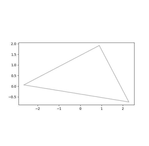
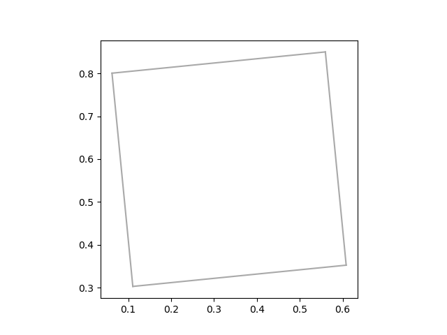
However, this results in a ValueError, as the shape of the output is incorrect. For the triangle example, the expected output shape is (3, 6), whereas the function above returns a (3, 2) array (i.e. 3 pairwise distance by 2 dimensions). For the square the expected output is (6, 8), whereas the actual is (6, 2). Any help deriving implementing the correct callable(s) for the jac arguments to NonlinearConstraint and minimize would be appreciated.

Note

I would like to avoid the use of autograd/jax/numdifftools (as in this question), as I would like to keep the number of dependencies of my library small.

Minimal working example(s)

#!/usr/bin/env python
"""
Create a node layout with fixed edge lengths but unknown node positions.
"""

import numpy as np

from scipy.optimize import minimize, NonlinearConstraint
from scipy.spatial.distance import pdist, squareform


def get_geometric_node_layout(edges, edge_length, node_size=0., power=0.2, maximum_iterations=200, origin=(0, 0), scale=(1, 1)):
    """Node layout for defined edge lengths but unknown node positions.

    Node positions are determined through non-linear optimisation: the
    total distance between nodes is maximised subject to the constraint
    imposed by the edge lengths, which are used as upper bounds.
    If provided, node sizes are used to set lower bounds.

    Parameters
    ----------
    edges : list
        The edges of the graph, with each edge being represented by a (source node ID, target node ID) tuple.
    edge_lengths : dict
        Mapping of edges to their lengths.
    node_size : scalar or dict, default 0.
        Size (radius) of nodes.
        Providing the correct node size minimises the overlap of nodes in the graph,
        which can otherwise occur if there are many nodes, or if the nodes differ considerably in size.
    power : float, default 0.2.
        The cost being minimised is the inverse of the sum of distances.
        The power parameter is the exponent applied to each distance before summation.
        Large values result in positions that are stretched along one axis.
        Small values decrease the influence of long distances on the cost
        and promote a more compact layout.
    maximum_iterations : int
        Maximum number of iterations of the minimisation.
    origin : tuple, default (0, 0)
        The (float x, float y) coordinates corresponding to the lower left hand corner of the bounding box specifying the extent of the canvas.
    scale : tuple, default (1, 1)
        The (float x, float y) dimensions representing the width and height of the bounding box specifying the extent of the canvas.

    Returns
    -------
    node_positions : dict
        Dictionary mapping each node ID to (float x, float y) tuple, the node position.

    """
    # TODO: assert triangle inequality

    # TODO: assert that the edges fit within the canvas dimensions

    # ensure that graph is bi-directional
    edges = edges + [(target, source) for (source, target) in edges] # forces copy
    edges = list(set(edges))

    # upper bound: pairwise distance matrix with unknown distances set to the maximum possible distance given the canvas dimensions
    lengths = []
    for (source, target) in edges:
        if (source, target) in edge_length:
            lengths.append(edge_length[(source, target)])
        else:
            lengths.append(edge_length[(target, source)])

    sources, targets = zip(*edges)
    nodes = sources + targets
    unique_nodes = set(nodes)
    indices = range(len(unique_nodes))
    node_to_idx = dict(zip(unique_nodes, indices))
    source_indices = [node_to_idx[source] for source in sources]
    target_indices = [node_to_idx[target] for target in targets]

    total_nodes = len(unique_nodes)
    max_distance = np.sqrt(scale[0]**2 + scale[1]**2)
    distance_matrix = np.full((total_nodes, total_nodes), max_distance)
    distance_matrix[source_indices, target_indices] = lengths
    distance_matrix[np.diag_indices(total_nodes)] = 0
    upper_bounds = squareform(distance_matrix)

    # lower bound: sum of node sizes
    if isinstance(node_size, (int, float)):
        sizes = node_size * np.ones((total_nodes))
    elif isinstance(node_size, dict):
        sizes = np.array([node_size[node] if node in node_size else 0. for node in unique_nodes])

    sum_of_node_sizes = sizes[np.newaxis, :] + sizes[:, np.newaxis]
    sum_of_node_sizes -= np.diag(np.diag(sum_of_node_sizes)) # squareform requires zeros on diagonal
    lower_bounds = squareform(sum_of_node_sizes)

    def cost_function(positions):
        return 1. / np.sum((pdist(positions.reshape((-1, 2))))**power)

    def constraint_function(positions):
        positions = np.reshape(positions, (-1, 2))
        return pdist(positions)

    initial_positions = _initialise_geometric_node_layout(edges)
    nonlinear_constraint = NonlinearConstraint(constraint_function, lb=lower_bounds, ub=upper_bounds, jac='2-point')
    result = minimize(cost_function, initial_positions.flatten(), method='SLSQP',
                      jac="2-point", constraints=[nonlinear_constraint], options=dict(maxiter=maximum_iterations))

    if not result.success:
        print("Warning: could not compute valid node positions for the given edge lengths.")
        print(f"scipy.optimize.minimize: {result.message}.")

    node_positions_as_array = result.x.reshape((-1, 2))
    node_positions = dict(zip(unique_nodes, node_positions_as_array))
    return node_positions


def _initialise_geometric_node_layout(edges):
    sources, targets = zip(*edges)
    total_nodes = len(set(sources + targets))
    return np.random.rand(total_nodes, 2)


if __name__ == '__main__':

    import matplotlib.pyplot as plt

    def plot_graph(edges, node_layout):
        # poor man's graph plotting
        fig, ax = plt.subplots()
        for source, target in edges:
            x1, y1 = node_layout[source]
            x2, y2 = node_layout[target]
            ax.plot([x1, x2], [y1, y2], color='darkgray')
        ax.set_aspect('equal')

    ################################################################################
    # triangle with right angle

    edges = [
        (0, 1),
        (1, 2),
        (2, 0)
    ]

    lengths = {
        (0, 1) : 3,
        (1, 2) : 4,
        (2, 0) : 5,
    }

    pos = get_geometric_node_layout(edges, lengths, node_size=0)

    plot_graph(edges, node_layout=pos)

    plt.show()

    ################################################################################
    # square

    edges = [
        (0, 1),
        (1, 2),
        (2, 3),
        (3, 0),
    ]

    lengths = {
        (0, 1) : 0.5,
        (1, 2) : 0.5,
        (2, 3) : 0.5,
        (3, 0) : 0.5,
    }

    pos = get_geometric_node_layout(edges, lengths, node_size=0)

    plot_graph(edges, node_layout=pos)

    plt.show()

Edit: Realistic use case for timing

Below is a more realistic use case that I am using to time my code. I have incorporated @adrianop01's computation of the Jacobian for the constraint. It also includes a superior initialisation. It requires the additional dependencies networkx and netgraph, both of which can be installed via pip.

#!/usr/bin/env python
"""
Create a node layout with fixed edge lengths but unknown node positions.
"""

import numpy as np

from itertools import combinations
from scipy.optimize import minimize, NonlinearConstraint
from scipy.spatial.distance import pdist, squareform

from netgraph._node_layout import _rescale_to_frame


def get_geometric_node_layout(edges, edge_length, node_size=0., power=0.2, maximum_iterations=200, origin=(0, 0), scale=(1, 1)):
    """Node layout for defined edge lengths but unknown node positions.

    Node positions are determined through non-linear optimisation: the
    total distance between nodes is maximised subject to the constraint
    imposed by the edge lengths, which are used as upper bounds.
    If provided, node sizes are used to set lower bounds.

    Parameters
    ----------
    edges : list
        The edges of the graph, with each edge being represented by a (source node ID, target node ID) tuple.
    edge_lengths : dict
        Mapping of edges to their lengths.
    node_size : scalar or dict, default 0.
        Size (radius) of nodes.
        Providing the correct node size minimises the overlap of nodes in the graph,
        which can otherwise occur if there are many nodes, or if the nodes differ considerably in size.
    power : float, default 0.2.
        The cost being minimised is the inverse of the sum of distances.
        The power parameter is the exponent applied to each distance before summation.
        Large values result in positions that are stretched along one axis.
        Small values decrease the influence of long distances on the cost
        and promote a more compact layout.
    maximum_iterations : int
        Maximum number of iterations of the minimisation.
    origin : tuple, default (0, 0)
        The (float x, float y) coordinates corresponding to the lower left hand corner of the bounding box specifying the extent of the canvas.
    scale : tuple, default (1, 1)
        The (float x, float y) dimensions representing the width and height of the bounding box specifying the extent of the canvas.

    Returns
    -------
    node_positions : dict
        Dictionary mapping each node ID to (float x, float y) tuple, the node position.

    """
    # TODO: assert triangle inequality

    # TODO: assert that the edges fit within the canvas dimensions

    # ensure that graph is bi-directional
    edges = edges + [(target, source) for (source, target) in edges] # forces copy
    edges = list(set(edges))

    # upper bound: pairwise distance matrix with unknown distances set to the maximum possible distance given the canvas dimensions
    lengths = []
    for (source, target) in edges:
        if (source, target) in edge_length:
            lengths.append(edge_length[(source, target)])
        else:
            lengths.append(edge_length[(target, source)])

    sources, targets = zip(*edges)
    nodes = sources + targets
    unique_nodes = set(nodes)
    indices = range(len(unique_nodes))
    node_to_idx = dict(zip(unique_nodes, indices))
    source_indices = [node_to_idx[source] for source in sources]
    target_indices = [node_to_idx[target] for target in targets]

    total_nodes = len(unique_nodes)
    max_distance = np.sqrt(scale[0]**2 + scale[1]**2)
    distance_matrix = np.full((total_nodes, total_nodes), max_distance)
    distance_matrix[source_indices, target_indices] = lengths
    distance_matrix[np.diag_indices(total_nodes)] = 0
    upper_bounds = squareform(distance_matrix)

    # lower bound: sum of node sizes
    if isinstance(node_size, (int, float)):
        sizes = node_size * np.ones((total_nodes))
    elif isinstance(node_size, dict):
        sizes = np.array([node_size[node] if node in node_size else 0. for node in unique_nodes])

    sum_of_node_sizes = sizes[np.newaxis, :] + sizes[:, np.newaxis]
    sum_of_node_sizes -= np.diag(np.diag(sum_of_node_sizes)) # squareform requires zeros on diagonal
    lower_bounds = squareform(sum_of_node_sizes)
    invalid = lower_bounds > upper_bounds
    lower_bounds[invalid] = upper_bounds[invalid] - 1e-8

    def cost_function(positions):
        # return -np.sum((pdist(positions.reshape((-1, 2))))**power)
        return 1. / np.sum((pdist(positions.reshape((-1, 2))))**power)

    def cost_jacobian(positions):
        # TODO
        pass

    def constraint_function(positions):
        positions = np.reshape(positions, (-1, 2))
        return pdist(positions)

    # adapted from https://mcmap.net/q/1342336/-how-to-compute-the-jacobian-of-a-pairwise-distance-function-scipy-spatial-pdist
    total_pairs = int((total_nodes - 1) * total_nodes / 2)
    source_indices, target_indices = np.array(list(combinations(range(total_nodes), 2))).T # node order thus (0,1) ... (0,N-1), (1,2),...(1,N-1),...,(N-2,N-1)
    rows = np.repeat(np.arange(total_pairs).reshape(-1, 1), 2, axis=1)
    source_columns = np.vstack((source_indices*2, source_indices*2+1)).T
    target_columns = np.vstack((target_indices*2, target_indices*2+1)).T

    def constraint_jacobian(positions):
        positions = np.reshape(positions, (-1, 2))
        pairwise_distances = constraint_function(positions)
        jac = np.zeros((total_pairs, 2 * total_nodes))
        jac[rows, source_columns] = (positions[source_indices] - positions[target_indices]) / pairwise_distances.reshape((-1, 1))
        jac[rows, target_columns] = -jac[rows, source_columns]
        return jac

    initial_positions = _initialise_geometric_node_layout(edges, edge_length)
    nonlinear_constraint = NonlinearConstraint(constraint_function, lb=lower_bounds, ub=upper_bounds, jac=constraint_jacobian)
    result = minimize(cost_function, initial_positions.flatten(), method='SLSQP',
                      jac='2-point', constraints=[nonlinear_constraint], options=dict(maxiter=maximum_iterations))
    # result = minimize(cost_function, initial_positions.flatten(), method='trust-constr',
    #                   jac=cost_jacobian, constraints=[nonlinear_constraint])

    if not result.success:
        print("Warning: could not compute valid node positions for the given edge lengths.")
        print(f"scipy.optimize.minimize: {result.message}.")

    node_positions_as_array = result.x.reshape((-1, 2))
    node_positions_as_array = _rescale_to_frame(node_positions_as_array, np.array(origin), np.array(scale))
    node_positions = dict(zip(unique_nodes, node_positions_as_array))
    return node_positions


# # slow
# def _initialise_geometric_node_layout(edges, edge_length=None):
#     sources, targets = zip(*edges)
#     total_nodes = len(set(sources + targets))
#     return np.random.rand(total_nodes, 2)

# much faster
def _initialise_geometric_node_layout(edges, edge_length=None):
    """Initialises the node positions using the FR algorithm with weights.
    Shorter edges are given a larger weight such that the nodes experience a strong attractive force."""

    from netgraph import get_fruchterman_reingold_layout
    if edge_length:
        edge_weight = dict()
        for edge, length in edge_length.items():
            edge_weight[edge] = 1 / length
    else:
        edge_weight = None
    node_positions = get_fruchterman_reingold_layout(edges)
    return np.array(list(node_positions.values()))


if __name__ == '__main__':

    from time import time
    import matplotlib.pyplot as plt
    import networkx as nx # pip install networkx

    from netgraph import Graph # pip install netgraph


    fig, (ax1, ax2) = plt.subplots(1, 2)

    g = nx.random_geometric_graph(50, 0.3, seed=2)
    node_positions = nx.get_node_attributes(g, 'pos')
    plot_instance = Graph(g,
                          node_layout=node_positions,
                          node_size=1, # netgraph rescales node sizes by 0.01
                          node_edge_width=0.1,
                          edge_width=0.1,
                          ax=ax1,
    )
    ax1.axis([0, 1, 0, 1])
    ax1.set_title('Original node positions')

    def get_euclidean_distance(p1, p2):
        return np.sqrt(np.sum((np.array(p1)-np.array(p2))**2))

    edge_length = dict()
    for (source, target) in g.edges:
        edge_length[(source, target)] = get_euclidean_distance(node_positions[source], node_positions[target])

    tic = time()
    new_node_positions = get_geometric_node_layout(list(g.edges), edge_length, node_size=0.01)
    toc = time()

    print(f"Time elapsed : {toc-tic}")

    Graph(g,
          node_layout=new_node_positions,
          node_size=1,
          node_edge_width=0.1,
          edge_width=0.1,
          ax=ax2,
    )
    ax2.axis([0, 1, 0, 1])
    ax2.set_title('Reconstructed node positions')

    plt.show()

---

2nd edit

Here are some preliminary results I obtained when testing @spinkus' and related solutions. My implementation of his code looks like this:

def cost_function(positions):
    return -np.sum((pdist(positions.reshape((-1, 2))))**2)

def cost_jacobian(positions):
    positions = positions.reshape(-1, 2)
    delta = positions[np.newaxis, :] - positions[:, np.newaxis]
    jac = -2 * np.sum(delta, axis=0)
    return jac.ravel()

Unfortunately, this cost function takes significantly longer to converge: 13 seconds in a best of 5 with a large variance in the timings (up to a minute). This is independent of whether I use the explicit Jacobian or approximate it using the finite difference approach. Furthermore, the minimisation often ends prematurely with "scipy.optimize.minimize: Inequality constraints incompatible." and "scipy.optimize.minimize: Positive directional derivative for linesearch." My bet (although I have little evidence to back it up) is that absolute value of the cost matters. My original cost function decreases both in value and in absolute value, whereas the minimisation increases the absolute value of the @spinkus cost function (however, see @spinkus' excellent comment below why that might be somewhat a red herring and lead to less accurate solutions).

I also understood (I think) why my original cost function is not amenable to computing the Jacobians. Let power be 0.5, then the cost function and Jacobian take this form (unless my algebra is wrong again):

def cost_function(positions):
    return 1. / np.sum((pdist(positions.reshape((-1, 2))))**0.5)

def cost_jacobian(positions):
    positions = positions.reshape(-1, 2)
    delta = positions[np.newaxis, :] - positions[:, np.newaxis]
    distance = np.sqrt(np.sum(delta**2, axis=-1))
    denominator = -2 * np.sqrt(delta) * distance[:, :, np.newaxis]
    denominator[np.diag_indices_from(denominator[:, :, 0]),:] = 1
    jac = 1 / denominator
    return np.sum(jac, axis=0).ravel() - 1

The problematic term is the sqrt(delta), where delta are the vectors between all points. Ignoring the diagonals, half of the entries in this matrix are necessarily negative and thus the Jacobian cannot be computed.

However, the purpose of the power is simply to decrease the importance of large distances on the cost. Any monotonically increasing function with decreasing derivative will do. Using log(x + 1) instead of the power results in these functions:

def cost_function(positions):
    return 1 / np.sum(np.log(pdist(positions.reshape((-1, 2))) + 1))

def cost_jacobian(positions):
    positions = positions.reshape(-1, 2)
    delta = positions[np.newaxis, :] - positions[:, np.newaxis]
    distance2 = np.sum(delta**2, axis=-1)
    distance2[np.diag_indices_from(distance2)] = 1
    jac = -delta / (distance2 + np.sqrt(distance2))[..., np.newaxis]
    return np.sum(jac, axis=0).ravel()

With the finite difference approximation, the minimisation terminates in 0.5 seconds. However, with the explicit Jacobian, the best run times were 4 seconds albeit still with a very large variance with run times up a minute and longer.

Tl;dr.

I still don't understand why the minimisation does not run faster with explicit Jacobians.

Graff

A quick question: Constraint_function(positions) should only calculate distances between point pairs with edges, not all points. Currently, this function is calculating dist between every possible point pair irrespective of whether there is an edge. Are you constraining all possible pairwise distances? Calculating the distance alone has a time complexity of O(n!) for n points, let along considering the time complexity of the later part of Jacobian calculations as well. – Unbutton

I do have an implementation of Jacobian in mind, but I think the program issue is the non-linear optimisation optimizing every pairwise point distance which has no relation to how the Jacobian is computed. I would suggest only constraining and optimizing the distances of points with edges. – Unbutton

@Unbutton Thank you for your comment. I am constraining all pairwise distances as I am using the lower bounds to prevent nodes overlapping with each other (irrespective of whether they are connected). The implementation is inspired by this SO answer. I could remove node overlaps in a second step. However, the cost function necessarily has to consider all pairwise distances, so this would remain a bottleneck either way. Also, the issue is not quite as dire as you make it out to be as there are not n! pairwise distances but just (n-1)*n / 2. – Graff

All that being said, I would be perfectly content with a solution that ignored the lower bounds and only considered connected nodes when applying the constraint. – Graff

You are right about the time complexity, did not realise that being nCr. – Unbutton

"... computes a set of N node positions for networks in which each edge has a defined length". I can't see an "edges have a defined length" constraint in code? Would "lengths constrained to a lower, upper bound" be accurate? – Katar

@Katar I believe it to be lower_bounds in OP's code – Unbutton

@Katar I set the upper bound for each pairwise distance to either the edge length (if there is one) or the length of the diagonal of the canvas, as defined by the scale parameter. – Graff

How do you know this problem is convex? Or are you happy just with a local minimum? – Katar

@Katar I don't think the problem is convex in general. However, I have a more complicated but much better way to initialize the node positions than in the code above (a similar method to the one I used here). From my experiments with simply using finite differences to approximate the Jacobians, I start the process reasonably close to the desired minimum such that finding a local minimum is sufficient for my purpose. – Graff

I see. Jacobian is relatively simple if you can make some simplifications like limiting power to 2 and changing the form of the objective from -1/x to -1x. Latter won't effect optimal. – Katar

@Katar The idea of using powers <<1 is to discount long distances and promote compact layouts. With larger powers, the node positions are typically arranged along one axis. I am hence somewhat reluctant on that front. – Graff

@Katar Changing the objective from -1/x to -1x is a great idea. However, from running a few simulations, finding a minimum takes longer (10x), at least when only using finite differences to approximate the Jacobians. But I guess all bets are off how fast it will be with explicit Jacobians. Looking forward to your solution. – Graff

I did not realise your second part (Jacobian for cost function) when I was writing my answer (my apologies). I do think an explicit Jacobian can be derived for your cost function unchanged, but I do agree with the answer of @Katar that a 2-norm-based cost function could be easier to derive and compute. Being very busy these days and would try to answer your second part (explicit Jacobian form of your original cost function) once I got some spare time. – Unbutton

Answer 1

I computed the the Jacobian ... However, ... ValueError ... Any help deriving implementing the correct callable(s) for the jac arguments to NonlinearConstraint and minimize would be appreciated.

Also stated:

power is a smallish number that limits the influence of large distances (to encourage compact node layouts) but for the purpose of this question could be assumed to be 1.

I said getting Jacobian was easy under assumptions in comments so ... here is an answer to explain what I meant. Disclaimer: in my testing code below is actually marginally slower than 2-point. On one hand, I could be wrong or made a mistake. On other hand, supposing the gradients are correct, it's not really surprising because 2-point is probably faster to calculate, the problem is highly constrained, convex only locally, and in most cases descends to a local minima in a short distance, so we might not benefit much from more accurate gradient info. If really want speed up maybe can look into lowering maxiter and ftol optimization settings. Answer:

Getting the Jacobian is simple when power is 1 or 2 - as shown in one of the Mathoverflow post you linked to - so I'm limited consideration to power = 2. Basically the Jacobian of the second norm of a vector (Latex: f(x) = ||x-c||_2^2) is just 2x (\nabla f(x) = \nabla ||x-c||_2^2 = 2x). You can probably generalize to power of any integer using the chain rule, just didn't consider it.

Restating the problem: We have a set of 2D points, X. We have a sub-graph G(V,E) where V is some subset of the points in X. An edge (a,b,l,u) in E implies the distance (assumed euclidean herein) between points a and b is between some constant values l, and u. We want to maximize the sum of the distance (to some power) between the points in X while satisfying the edge constraints given by G. I'm also assuming all points in X are bound to [0,1]. I.e objective is:

Let |X| = N. f is a function f:R^{2N}->R, and the "Jacobian" in this case is just the gradient vector of f (a vector in R^{2N}). If we consider just two points, X = {a,b} it's easy to see the gradient is parallel to the edge between those two points:

When power is positive the gradient points outward (as above). When it's negative it points inward. The magnitude depends on power. When p = 2 it's just +/- the edge vector times two for a and b (when p = 1 it's just +/- the given unit vector). Extending to more points the gradient for some a in X, is just the sum of all those vectors for each other point:

Code:

I'm going to assume power = 2 as stated, and use the -1x form not -1/x. Both assumptions make the gradient easier to derive:

import os
import numpy as np
import matplotlib.pyplot as plt
from scipy.optimize import minimize, Bounds
from scipy.spatial import distance_matrix

# Numer of nodes:
n = 4
points = np.random.random((n,2))*.8+0.1
# Random sparse edges between points:
adj_matrix = np.triu(np.random.randint(0, 2, (n,n)), 1)*np.triu(np.random.randint(0, 2, (n,n)), 1)
adj_list = [(i, j) for (i, x) in enumerate(adj_matrix) for (j,y) in enumerate(x) if y == 1]
# Upper/lower bound for points in adj_list is initial distance +/- slack/2:
slack = 5e-3
# Initial distance matrix squared. Used for edge constraints:
point_distances = distance_matrix(points, points)**2


def cost_function(x):
  return -1 * distance_matrix(x.reshape((-1,2)), x.reshape((-1,2))**2).sum()/2.


def deriv_function(x):
  return -2 * (n * x.reshape((-1,2)) - x.reshape((-1,2)).sum(axis=0))


def constraints():
  def zmm(x, keep, axis=0, fn=None):
    ''' Zero mask out rows/cols along axis not in keep index, applying fn(<kept>) if fn is provided.
    I couldn't find this in Numpy.
    '''
    r = np.zeros(x.shape)
    if axis == 0:
      i = x[keep,:]
      r[keep,:] = fn(i).reshape(i.shape) if fn else i
    elif axis == 1:
      i = x[:,keep]
      r[:,keep] = fn(i).reshape(i.shape) if fn else i
    else:
      raise np.AxisError(axis)
    return r
  # NOTE: Added scaling factor due to getting "Positive directional derivative for linesearch".
  # I don't completely understand it but means either scaling issue, or jac is wrong, or SLSQP just sucks.
  # See https://mcmap.net/q/628236/-positive-directional-derivative-for-linesearch
  k=1e-3
  constraints = []
  for (i,j) in adj_list:
    constraints += [{
      'type': 'ineq',
      'fun': lambda x, i=i, j=j: k * (((x.reshape((-1,2))[j] - x.reshape((-1,2))[i])**2).sum() - point_distances[i,j] + slack),
      'jaq': lambda x, i=i, j=j: 2 * k * (lambda x=x.reshape((-1,2)): zmm(x, i, lambda v: x[j] - x[i]) - zmm(x, j, lambda v: x[j] - x[i]))(x)
    }]
    constraints += [{
      'type': 'ineq',
      'fun': lambda x, i=i, j=j: k * (point_distances[i,j] - ((x.reshape((-1,2))[j] - x.reshape((-1,2))[i])**2).sum()  + slack),
      'jaq': lambda x, i=i, j=j: -2 * k * (lambda x=x.reshape((-1,2)): zmm(x, i, lambda v: x[j] - x[i]) - zmm(x, j, lambda v: x[j] - x[i]))(x)
    }]
  return constraints

solver_options = {
  'ftol': 1e-3,
  'maxiter': 1e2,
  'disp': True
}

result = minimize(
  cost_function,
  points.flatten(),
  method='SLSQP',
  jac=deriv_function,
  bounds=Bounds(0,1),
  constraints=constraints(),
  options=solver_options
)
soln = result.x.reshape((-1,2))
print(result)
print('Improvement:', cost_function(points)- cost_function(soln))

if 'SHOW_PLOTS' in os.environ:

  fig, axes = plt.subplots(nrows=1, ncols=2)
  ax0, ax1 = axes.flatten()
  ax0.scatter(points[:,0], points[:,1])
  for (i,j) in adj_list:
    ax0.plot([points[i][0], points[j][0]], [points[i][1], points[j][1]], 'go-')
  ax1.scatter(soln[:,0], soln[:,1])
  for (i,j) in adj_list:
    ax1.plot([soln[i][0], soln[j][0]], [soln[i][1], soln[j][1]], 'go-')
  ax0.set_xlim(-0.1,1.1)
  ax0.set_ylim(-0.1,1.1)
  ax1.set_xlim(-0.1,1.1)
  ax1.set_ylim(-0.1,1.1)
  ax0.set_xticks(np.linspace(0,1,5))
  ax0.set_yticks(np.linspace(0,1,5))
  ax1.set_xticks(np.linspace(0,1,5))
  ax1.set_yticks(np.linspace(0,1,5))
  ax0.set_aspect('equal', 'box')
  ax1.set_aspect('equal', 'box')
  plt.show()

Results (random edge constraints; before/after):

n=12:

n=4:

Katar

Thank you for your very intuitive explanation. That was very helpful. Unfortunately, the choice of cost function seems to hinder convergence in my test case, as it increases the time to convergence substantially (13 seconds in a best of 5 with a large variance with and without using the explicit Jacobians compared to 0.7 seconds when using my attempt). – Graff

Just to cost function form? Interesting. In my testing over 30 trials at n=20 the 1/x form is about twice as fast as -1x. However, I can make one slower and the other faster by changing the scaling factor to the point where they are about the same. This leads me to suspect one just satisfies a stopping criteria earlier - with less accurate solution. Only other thing is I used distance_matrix over pdist but I don't think that would account for a large difference. – Katar

That is a good point. As the absolute value decreases in my original cost function, the minimisation should terminate earlier given the same ftol. Visually, however, the solutions look pretty good when I use 1/x and variants thereof. FYI: I have tested some more cost functions. see my second edit above. – Graff

Answer 2

This implementation calculates the Jacobian for the constraint function, for all point pairs according to the discussion with OP. The np array vectorization code may not be perfect, thus I welcome further comments for code refinement based on the Jacobian formula.

Derivation of Jacobian Matrix

2d Point can be defined as a vector:

Jacobian matrix is (M rows, N columns, M is the number of unique 2-point pairs, N is the number of unique points):

For each individual element of the Jacobian matrix, we have the following three cases:

1. The specific point coordinate x/y is point 1 x/y in the 2-norm.
2. The specific point coordinate x/y is point 2 x/y in the 2-norm.
3. The specific point coordinate x/y does not relate to the current 2-norm.

Thus, we would expect the Jacobian to be a sparse matrix with lots of zeros with at most 4 non-zero entries per row.

Code

The code is self-explanatory. We start the Jacobian as an MxN np.zeros matrix, and only update those entries that are related to the current 2 norm function/point pair (thus, 4 updates per row).

from itertools import combinations

n_pt = len(initial_positions) #N
n_ptpair = len(upper_bounds) #total number of pointpairs, M

idx_pts= np.array(list(combinations(range(n_pt),2))) #point id order thus in (0,1) ... (0,N-1), (1,2),...(1,N-1),...,(N-2,N-1)
idx_pt1= np.array(idx_pts[:,0]) 
idx_pt2= np.array(idx_pts[:,1])

row_idx = np.repeat(np.arange(n_ptpair).reshape(-1,1),2,axis=1)
col1_idx = np.vstack((idx_pt1*2,idx_pt1*2+1)).T
col2_idx = np.vstack((idx_pt2*2,idx_pt2*2+1)).T

def delta_constraint(positions):
  positions = np.reshape(positions, (-1, 2))
  pairdist = constraint_function(positions) #pairwise R2 distance between each point pair
  jac = np.zeros((n_ptpair,2*n_pt)) #(M,(x0,y0,x1,y1,...,xc,yc...,xN,yN))
  jac[row_idx,col1_idx] = (positions[idx_pt1]-positions[idx_pt2])/pairdist.reshape((-1,1))
  jac[row_idx,col2_idx] = -jac[row_idx,col1_idx]
  return jac

Results

1.Triangle in your code

2.Square in your code

3.A rather complicated graph

  edges = [
        (0, 1),
        (1, 2),
        (2, 3),
        (3, 0),
        (3, 1),
        (4, 1),
        (5, 1),
        (5, 2),
    ]

    lengths = {
        (0, 1) : 0.5,
        (1, 2) : 0.5,
        (2, 3) : 0.5,
        (3, 0) : 0.5,
        (3, 1) : 0.8,
        (4, 1) : 0.8,
        (5, 1) : 0.2,
        (5, 2) : 1,
    }

Unbutton

The jacobian is pretty sparse as you already mentioned, so using a sparse data structure like scipy.sparse.coo_array would be way more efficient and makes the evaluation of the jacobian function faster. However, it's worth mentioning that scipy's implementation of the 'SLSQP' algorithm doesn't support sparse jacobians yet, IIRC only 'trust-constrs' does. – Your

I will award the current bounty to your answer once the 24h grace period expires, and then create another bounty to hopefully attract an answer to the second part of my question, i.e. computing the Jacobian for the cost function. – Graff