Speed difference of loop Inside vs Outside Function

Question

Out of this SO post resulted a discussion when benchmarking the various solutions. Consider the following code

# global environment is empty - new session just started
# set up
set.seed(20181231)
n <- sample(10^3:10^4,10^3)
for_loop <- function(n) {
  out <- integer(length(n))
  for(k in 1:length(out)) {
    if((k %% 2) == 0){
      out[k] <- 0L
      next
    }
    out[k] <- 1L
    next
  }
  out
}
# benchmarking
res <- microbenchmark::microbenchmark(
  for_loop = {
    out <- integer(length(n))
    for(k in 1:length(out)) {
      if((k %% 2) == 0){
        out[k] <- 0L
        next
      }
      out[k] <- 1L
      next
    }
    out
  },
  for_loop(n),
  times = 10^4
)

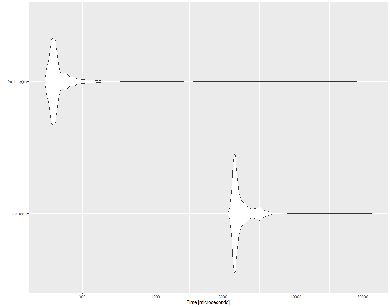
Here are the benchmarking results for the exact same loops, one packed in a function, the other not

# Unit: microseconds
#        expr      min       lq      mean   median       uq      max neval cld
#    for_loop 3216.773 3615.360 4120.3772 3759.771 4261.377 34388.95 10000   b
# for_loop(n)  162.280  180.149  225.8061  190.724  211.875 26991.58 10000  a 
ggplot2::autoplot(res)

As can be seen, there is a drastic difference in efficiency. What is the underlying reason for this?

To be clear, the question is not about the task solved by the above code (which could be done much more elegantly) but merely about efficiency discrepancy between a regular loop and a loop wrapped inside a function.

Holusbolus

I understand. I did however empty my environment and restarted a new session before every trial, so the only variable extra in the global environment is for_loop. Do you believe it could still be the reason behind that lag? – Holusbolus

I've deleted that comment; the real reason is in my answer below. – Peaceful

Answer 1

The explanation is that functions are "just-in-time" compiled, whereas interpreted code is not. See ?compiler::enableJIT for a description.

If you want a demonstration of the difference, run

compiler::enableJIT(0)

before any of your code (including the creation of the for_loop function). This disables JIT compiling for the rest of that session. Then the timing will be much more similar for the two sets of code.

You have to do this before the creation of the for_loop function, because once it gets compiled by the JIT compiler, it will stay compiled, whether JIT is enabled or not.

Peaceful

That's interesting. But I am a little bit lost with the with/without function: you are saying "the 'with function' version took longer: there's more overhead being measured". But didn't the result indicate the reverse? – Holusbolus

My explanation was a mess; sorry. I've rewritten it to be a lot clearer. – Peaceful

Thanks, that helps. I've tested with compiler::enableJIT(0) and just like you said the results were similar (~2.2 millis.). How should interpret the first microbenchmark results? Are those faster results "cheated" or "not real"? – Holusbolus

As far as I know they're fine, it was my alternate timing code that was wrong, so I've deleted that. – Peaceful

What I meant was compiler::enableJIT(3) (default) and compiler::enableJIT(0) yield different benchmarking results (~4k and~200 micro. for the former and ~2.4k and ~2.2k micro. for the latter - using microbenchmark). So my questions: Which benchmarks are more meaningful? Is the ~200 micro. benchmark "real" or is it omitting computation time that would actually occur when running the code in a program? – Holusbolus

It will only count the compilation time once. If your program only calls the function a few times instead of 10000 times, compilation time will matter a lot more. – Peaceful