Override lower, upper, etc. in boxplot while grouping

Per default, for the lower, middle and upper quantile in geom_boxplot the 25%-, 50%-, and 75%-quantiles are considered. These are computed from y, but can be set manually via the aesthetic arguments lower, upper, middle (providing also x, ymin and ymax and setting stat="identity").

However, doing so, several undesirable effects occur (cf. version 1 in the example code):

The argument group is ignored, so all values of a column are considered in calculations (for instance when computing the lowest quantile for each group)
The resulting identical boxplots are grouped by x, and repeated within the group as often as the specific group value occurs in the data (instead of merging the boxes to a wider one)
outliers are not plotted

By pre-computing the desired values and storing them in a new data frame, one can handle the first two points (cf. version 2 in the example code), while the third point is fixed by identifying the outliers and adding them separately to the chart via geom_point.

Is there a more straight forward way to have the quantiles changed, without having these undesired effects?

Example Code:

set.seed(12)

# Random data in B, grouped by values 1 to 4 in A
u <- data.frame(A = sample.int(4, 100, replace = TRUE), B = rnorm(100))

# Desired arguments
qymax <- 0.9
qymin <- 0.1
qmiddle <- 0.5
qupper <- 0.8
qlower <- 0.2

Version 1: Repeated boxplots per value in A, grouped by A

ggplot(u, aes(x = A, y = B)) + 
  geom_boxplot(aes(group=A, 
                   lower = quantile(B, qlower), 
                   upper = quantile(B, qupper), 
                   middle = quantile(B, qmiddle), 
                   ymin = quantile(B, qymin), 
                   ymax = quantile(B, qymax) ), 
               stat="identity")

Version 2: Compute the arguments first for each group. Base R solution

Bgrouped <- lapply(unique(u$A), function(a) u$B[u$A == a])
.lower <- sapply(Bgrouped, function(x) quantile(x, qlower))
.upper <- sapply(Bgrouped, function(x) quantile(x, qupper))
.middle <- sapply(Bgrouped, function(x) quantile(x, qmiddle))
.ymin <- sapply(Bgrouped, function(x) quantile(x, qymin))
.ymax <- sapply(Bgrouped, function(x) quantile(x, qymax))

u <- data.frame(A = unique(u$A), 
                lower = .lower, 
                upper = .upper, 
                middle = .middle, 
                ymin = .ymin, 
                ymax = .ymax)    

ggplot(u, aes(x = A)) + 
  geom_boxplot(aes(lower = lower, upper = upper, 
                   middle = middle, ymin = ymin, ymax = ymax ), 
               stat="identity")

It's not something I'd really do without a lot of justification, as people typically expect the boxplot's min / max / box values to correspond to the same quantile positions, but it can be done.

Data used (with extreme values added to demonstrate outliers):

set.seed(12)
u <- data.frame(A = sample.int(4, 100, replace = TRUE), B = rnorm(100))
u$B[c(30, 70, 76)] <- c(4, -4, -5)

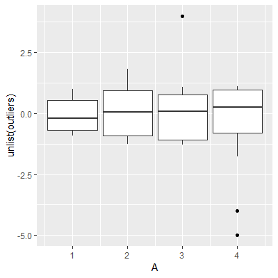
Solution 1: You can pre-compute the values without going by the base R route, & include calculations for outliers in the same step. I'd do it completely within Hadley's tidyverse libraries, which I find neater:

library(dplyr)
library(tidyr)

u %>%
  group_by(A) %>%
  summarise(lower = quantile(B, qlower),
            upper = quantile(B, qupper), 
            middle = quantile(B, qmiddle), 
            IQR = diff(c(lower, upper)),
            ymin = max(quantile(B, qymin), lower - 1.5 * IQR), 
            ymax = min(quantile(B, qymax), upper + 1.5 * IQR),
            outliers = list(B[which(B > upper + 1.5 * IQR | 
                                      B < lower - 1.5 * IQR)])) %>%
  ungroup() %>% 
  ggplot(aes(x = A)) + 
  geom_boxplot(aes(lower = lower, upper = upper,
                   middle = middle, ymin = ymin, ymax = ymax ),
               stat="identity") + 
  geom_point(data = . %>% 
               filter(sapply(outliers, length) > 0) %>%
               select(A, outliers) %>%
               unnest(), 
             aes(y = unlist(outliers)))

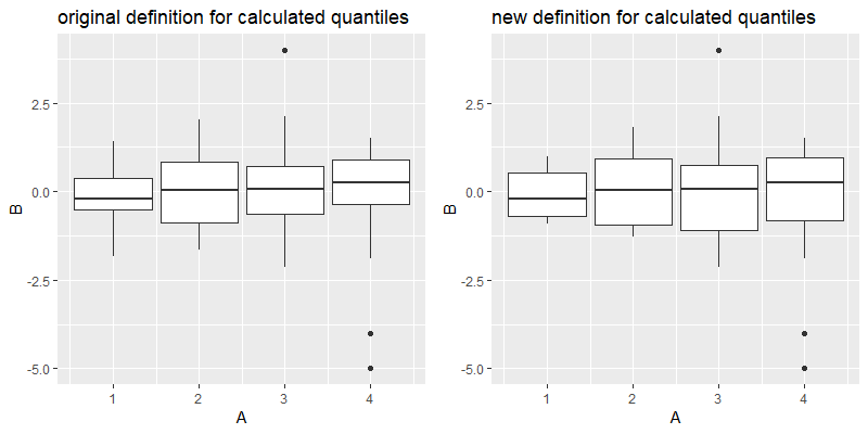
Solution 2: You can override the actual quantile specifications used by ggplot. The calculations for geom_boxplot()'s quantiles are actually in StatBoxplot's compute_group() function, found here:

compute_group = function(data, scales, width = NULL, na.rm = FALSE, coef = 1.5) {
    qs <- c(0, 0.25, 0.5, 0.75, 1)

    if (!is.null(data$weight)) {
      mod <- quantreg::rq(y ~ 1, weights = weight, data = data, tau = qs)
      stats <- as.numeric(stats::coef(mod))
    } else {
      stats <- as.numeric(stats::quantile(data$y, qs))
    }

... (omitted for space)

The qs vector defines the quantile positions. It's not affected by parameters passed to compute_group(), so the only way to change that is to change the definition for compute_group() itself:

# save a copy of the original function, in case you need to revert
original.function <- environment(ggplot2::StatBoxplot$compute_group)$f

# define new function (only the first line for qs is changed, but you'll have to
# copy & paste the whole thing)
new.function <- function (data, scales, width = NULL, na.rm = FALSE, coef = 1.5) {
  qs <- c(0.1, 0.2, 0.5, 0.8, 0.9)
  if (!is.null(data$weight)) {
    mod <- quantreg::rq(y ~ 1, weights = weight, data = data, 
                        tau = qs)
    stats <- as.numeric(stats::coef(mod))
  }
  else {
    stats <- as.numeric(stats::quantile(data$y, qs))
  }
  names(stats) <- c("ymin", "lower", "middle", "upper", "ymax")
  iqr <- diff(stats[c(2, 4)])
  outliers <- data$y < (stats[2] - coef * iqr) | data$y > (stats[4] + 
                                                             coef * iqr)
  if (any(outliers)) {
    stats[c(1, 5)] <- range(c(stats[2:4], data$y[!outliers]), 
                            na.rm = TRUE)
  }
  if (length(unique(data$x)) > 1) 
    width <- diff(range(data$x)) * 0.9
  df <- as.data.frame(as.list(stats))
  df$outliers <- list(data$y[outliers])
  if (is.null(data$weight)) {
    n <- sum(!is.na(data$y))
  }
  else {
    n <- sum(data$weight[!is.na(data$y) & !is.na(data$weight)])
  }
  df$notchupper <- df$middle + 1.58 * iqr/sqrt(n)
  df$notchlower <- df$middle - 1.58 * iqr/sqrt(n)
  df$x <- if (is.factor(data$x)) 
    data$x[1]
  else mean(range(data$x))
  df$width <- width
  df$relvarwidth <- sqrt(n)
  df
}

Result:

# toggle between the two definitions
environment(StatBoxplot$compute_group)$f <- original.function
ggplot(u, aes(x = A, y = B, group = A)) +
  geom_boxplot() +
  ggtitle("original definition for calculated quantiles")

environment(StatBoxplot$compute_group)$f <- new.function
ggplot(u, aes(x = A, y = B, group = A)) +
  geom_boxplot() +
  ggtitle("new definition for calculated quantiles")

Do note that when you change the definition, it affects every ggplot object in your environment. So if you've created a ggplot boxplot object before the definition change, & print it out afterwards, the boxplot will follow the new definition. (For the side-by-side comparison above, I had to convert each ggplot to a grob object immediately, in order to preserve the difference.)

Recommended topics

Hot tags