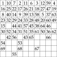
First of all:
What is going on here?
To see what is happening, here are PostScript definitions that let us visualize the search:
/n 5 def

340 n div dup scale
-0.9 0.1 translate % leave room for line strokes

/Palatino-Roman 0.8 selectfont

/coords { n exch sub translate } bind def

/num { 3 1 roll gsave coords 0.5 0.2 translate
    5 string cvs dup stringwidth pop -2 div 0 moveto show
    grestore } bind def

/clr { gsave coords 1 setgray 0 0 1 1 4 copy rectfill
     0 setgray 0.02 setlinewidth rectstroke grestore} bind def

1 1 n { 1 1 n { 1 index clr } for pop } for
These definitions give you two procedures:
clr to clear a squarenum to show a number on a square.
For example, if you save these definitions to tour.ps and then invoke the PostScript interpreter Ghostscript with:
gs -r72 -g350x350 tour.ps
and then enter the following instructions:
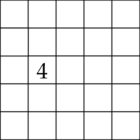
1 2 3 num
1 2 clr
2 3 4 num
you get:
![PostScript sample instructions]()
PostScript is a great programming language for visualizing search processes, and I also recommend to check out postscript for more information.
We can easily modify your program to emit suitable PostScript instructions that let us directly observe the search. I highlight the relevant additions:
constrain_entries([], _Square, _X, _Y).
constrain_entries([E|Es], Square, X, Y) :-
    freeze(E, postscript(X, Y, E)),
    constrain_entry(E, Square, X, Y),
    X1 #= X + 1,
    constrain_entries(Es, Square, X1, Y).

postscript(X, Y, N) :- format("~w ~w ~w num\n", [X,Y,N]).
postscript(X, Y, _) :- format("~w ~w clr\n", [X,Y]), false.
I have also taken the liberty to change (is)/2 to (#=)/2 to make the program more general.
Assuming that you saved the PostScript definitions in tour.ps and your Prolog program in tour.pl, the following invocation of SWI-Prolog and Ghostscript illustrates the situation:
swipl -g "number_puzzle_(_, Vs), label(Vs)" tour.pl | gs -g350x350 -r72 tour.ps -dNOPROMPT
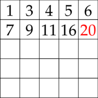
For example, we see a lot of backtracking at the highlighted position:
![Thrashing illustration]()
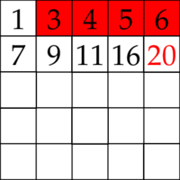
However, essential problems already lie completely elsewhere:
![Thrashing reason]()
None of the highlighted squares are valid moves!
From this, we see that your current formulation does not—at least not sufficiently early—let the solver recognize when a partial assignment cannot be completed to a solution! This is bad news, since failure to recognize inconsistent assignments often leads to unacceptable performance. For example, in order to correct the 1 → 3 transition (which can never occur in this way, yet is already one of the first choices made in this case), the solver would have to backtrack over approximately 8 squares, after enumerating—as a very rough estimate—258 = 152587890625 partial solutions, and then start all over at only the second position in the board.
In the constraint literature, such backtracking is called thrashing. It means repeated failure due to the same reason.
How is this possible? Your model seems to be correct, and can be used to detect solutions. That's good! However, a good constraint formulation not only recognizes solutions, but also quickly detects partial assignments that cannot be completed to solutions. This is what allows the solver to effectively prune the search, and it is in this important respect that your current formulation falls short. One of the reasons for this has to do with constraint propagation in reified constraints that you are using. In particular, consider the following query:
?- (X + 1 #= 3) #<==> B, X #\= 2.
Intuitively, we expect B = 0. But that is not the case! Instead, we get:
X in inf..1\/3..sup,
X+1#=_3840,
_3840#=3#B,
B in 0..1.
So, the solver does not propagate reified equality very strongly. Maybe it should though! Only sufficient feedback from Prolog practitioners will tell whether this area of the constraint solver should be changed, possibly trading a bit of speed for stronger propagation. The high relevance of this feedback is one of the reasons why I recommend to use CLP(FD) constraints whenever you have the opportunity, i.e., every time you are reasoning about integers.
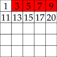
For this particular case, I can tell you that making the solver stronger in this sense does not make that much of a difference. You essentially end up with a version of the board where the core issue still arises, with many transitions (some of them highlighted below) that cannot occur in any solution:
![Thrashing also with domain consistency]()
Fixing the core issue
We should eliminate the cause of the backtracking at its core. To prune the search, we must recognize inconsistent (partial) assignments earlier.
Intuitively, we are searching for a connected tour, and want to backtrack as soon as it is clear that the tour cannot be continued in the intended way.
To accomplish what we want, we have at least two options:
- change the allocation strategy to take connectedness into account
- model the problem in such a way that connectedness is more strongly taken into account.
Option 1: Allocation strategy
A major attraction of CLP(FD) constraints is that they let us decouple the task description from the search. When using CLP(FD) constraints, we often perform search via label/1 or labeling/2. However, we are free to assign values to variables in any way we want. This is very easy if we follow—as you have done—the good practice of putting the "constraint posting" part into its own predicate, called the core relation.
For example, here is a custom allocation strategy that makes sure that the tour remains connected at all times:
allocation(Vs) :-
        length(Vs, N),
        numlist(1, N, Ns),
        maplist(member_(Vs), Ns).

member_(Es, E) :- member(E, Es).
With this strategy, we get a solution for the 5×5 instance from scratch:
?- number_puzzle_(Square, Vars), time(allocation(Vars)).
% 5,030,522 inferences, 0.907 CPU in 0.913 seconds (99% CPU, 5549133 Lips)
Square = square(row(1, 8, 5, 2, 11), ...),
Vars = [1, 8, 5, 2, 11, 16, 21, 24, 15|...]
There are various modifications of this strategy that are worth trying out. For example, when multiple squares are admissible, we could try to make a more intelligent choice by taking into account the number of remaining domain elements of the squares. I leave trying such improvements as a challenge.
From the standard labeling strategies, the min labeling option is in effect quite similar to this strategy in this case, and indeed it also finds a solution for the 5×5 case:
?- number_puzzle_(Square, Vars), time(labeling([min], Vars)).
% 22,461,798 inferences, 4.142 CPU in 4.174 seconds (99% CPU, 5422765 Lips)
Square = square(row(1, 8, 5, 2, 11), ...),
Vars = [1, 8, 5, 2, 11, 16, 21, 24, 15|...] .
However, even a fitting allocation strategy cannot fully compensate weak constraint propagation. For the 10×10 instance, the board looks like this after some search with the min option:
![Thrashing with labeling option <code>min</code>]()
Note that we also have to adapt the value of n in the PostScript code to visualize this as intended.
Ideally, we should formulate the task in such a way that we benefit from strong propagation, and then also use a good allocation strategy.
Option 2: Remodeling
A good CLP formulation propagates as strongly as possible (in acceptable time). We should therefore strive to use constraints that allow the solver to reason more readily about the task's most important requirements. In this concrete case, it means that we should try to find a more suitable formulation for what is currently expressed as a disjunction of reified constraints that, as shown above, do not allow much propagation. In theory, the constraint solver could recognize such patterns automatically. However, that is impractical for many use cases, and we therefore must sometimes experiment by manually trying several promising formulations. Still, also in this case: With sufficient feedback from application programmers, such cases are more likely to be improved and worked on!
I now use the CLP(FD) constraint circuit/1 to make clear that we are looking for a Hamiltonian circuit in a particular graph. The graph is expressed as a list of integer variables, where each element denotes the position of its successor in the list.
For example, a list with 3 elements admits precisely 2 Hamiltonian circuits:
?- Vs = [_,_,_], circuit(Vs), label(Vs).
Vs = [2, 3, 1] ;
Vs = [3, 1, 2].
I use circuit/1 to describe solutions that are also closed tours. This means that, if we find such a solution, then we can start again from the beginning via a valid move from the last square in the found tour:
n_tour(N, Vs) :-
        L #= N*N,
        length(Vs, L),
        successors(Vs, N, 1),
        circuit(Vs).

successors([], _, _).
successors([V|Vs], N, K0) :-
        findall(Num, n_k_next(N, K0, Num), [Next|Nexts]),
        foldl(num_to_dom, Nexts, Next, Dom),
        V in Dom,
        K1 #= K0 + 1,
        successors(Vs, N, K1).

num_to_dom(N, D0, D0\/N).

n_x_y_k(N, X, Y, K) :- [X,Y] ins 1..N, K #= N*(Y-1) + X.

n_k_next(N, K, Next) :-
        n_x_y_k(N, X0, Y0, K),
        (   [DX,DY] ins -2 \/ 2
        ;   [DX,DY] ins -3 \/ 0 \/ 3,
            abs(DX) + abs(DY) #= 3
        ),
        [X,Y] ins 1..N,
        X #= X0 + DX,
        Y #= Y0 + DY,
        n_x_y_k(N, X, Y, Next),
        label([DX,DY]).
Note how admissible successors are now expressed as domain elements, reducing the number of constraints and entirely eliminating the need for reifications. Most importantly, the intended connectedness is now automatically taken into account and enforced at every point during the search. The predicate n_x_y_k/4 relates (X,Y) coordinates to list indices. You can easily adapt this program to other tasks (e.g., knight's tour) by changing n_k_next/3. I leave the generalization to open tours as a challenge.
Here are additional definitions that let us print solutions in a more readable form:
:- set_prolog_flag(double_quotes, chars).

print_tour(Vs) :-
        length(Vs, L),
        L #= N*N, N #> 0,
        length(Ts, N),
        tour_enumeration(Vs, N, Es),
        phrase(format_string(Ts, 0, 4), Fs),
        maplist(format(Fs), Es).

format_(Fs, Args, Xs0, Xs) :- format(chars(Xs0,Xs), Fs, Args).

format_string([], _, _) --> "\n".
format_string([_|Rest], N0, I) -->
        { N #= N0 + I },
        "~t~w~", call(format_("~w|", [N])),
        format_string(Rest, N, I).

tour_enumeration(Vs, N, Es) :-
        length(Es, N),
        maplist(same_length(Es), Es),
        append(Es, Ls),
        foldl(vs_enumeration(Vs, Ls), Vs, 1-1, _).

vs_enumeration(Vs, Ls, _, V0-E0, V-E) :-
        E #= E0 + 1,
        nth1(V0, Ls, E0),
        nth1(V0, Vs, V).
In formulations with strong propagation, the predefined ff search strategy is often a good strategy. And indeed it lets us solve the whole task, i.e., the original 10×10 instance, within a few seconds on a commodity machine:
?- n_tour(10, Vs),
   time(labeling([ff], Vs)),
   print_tour(Vs).
% 5,642,756 inferences, 0.988 CPU in 0.996 seconds (99% CPU, 5710827 Lips)
   1  96  15   2  97  14  80  98  13  79
  93  29  68  94  30  27  34  31  26  35
  16   3 100  17   4  99  12   9  81  45
  69  95  92  28  67  32  25  36  33  78
  84  18   5  83  19  10  82  46  11   8
  91  23  70  63  24  37  66  49  38  44
  72  88  20  73   6  47  76   7  41  77
  85  62  53  86  61  64  39  58  65  50
  90  22  71  89  21  74  42  48  75  43
  54  87  60  55  52  59  56  51  40  57
Vs = [4, 5, 21, 22, 8, 3, 29, 26, 6|...]
For utmost performance, I recommend you also try this with other Prolog systems. The efficiency of commercial-grade CLP(FD) systems is often an important reason for buying a Prolog system.
Note also that this is by no means the only promising Prolog or even CLP(FD) formulation of the task, and I leave thinking about other formulations as a challenge.

